[COMPSCI 180] Project F: NeRF

8 minute read

Published: December 12, 2024

Implementing NeRF

Introduction

NeRF is a novel scene synthesis technique first proposed by Mildenhall et al., which attempts to visualize complex geometries at high resolutions via three main methodological features:

March camera rays through a scene to first generated sampled set of 3D points.
Using those points and their corresponding 2D viewing directions, represented by extrinsic matrices (camera viewpoints), one can try to predict the density and color of a specific point.
Lastly, to transform the density and colors of pixels into a scene representation, NeRF uses classical volumetric rendering techniques to accumulate the colors and densities into 2-dimensional images.

Several of these approaches are powered by MLPs.

For this precanned final project of COMSPCI 180, we aim to implement an easier version of NeRF.

Methods

Building a 2D Neural Field

A vector field is essentially a function that maps each n-dimensional coordinate to a vector. A neural field, temrinologically similar, is a neural network architecture that maps some n-dimensional coordinate to a particular 3-dimensional datapoint that represents its color. Fundamentally, we train a neural network $F: (x, y) \rightarrow (r, g, b)$ to predict the color of each pixel on an image.

As an exercise, let us discuss how to build such neural fields in the easiest case like for a two-dimensional image. In NeRF, a similar approach is taken: a three-dimensional world coordinate and a two-dimensional representation of the camera viewing direction are used as the input of a neural network to output the color of a pixel (along with its density, but let us abstract this away first). However, as NeRF has mentioned, prior works have failed replicating high-frequency details of an image with this approach. To allow for this variability, we need the field to be constructed with higher-dimensional inputs.

To construct higher-dimensional inputs from low-dimensional points, we introduce positional encoding. Simply put, it’s an expanded representation of some low-dimensional point. In our implementation, we use the following:

\[PE(x) = \{x, \sin(2^0 \pi x), \cos(2^0 \pi x), \cdots, \sin(2^{L-1} \pi x), \cos(2^{L-1} \pi x)\}\]

where the hyperparameter $L$ controls the dimensionality of our expanded representation. This is similar to the samely named idea used in transformer architectures.

Therefore, to train a 2D neural field that predicts the color of any pixel in a 2D image, we will first train the neural field on the 2D image per se, and use the MSE of the predicted and true color of each pixel as the training objective. Additionally, we evaluate our results via the metric Peak Signal-to-Noise Ratio (PSNR), formulated as follows:

\[{\rm PSNR} = 10 \log_{10} \bigg( \frac{1}{\rm MSE} \bigg)\]

Pixel, Camera, World

In the 2D neural field, each pixel is one pair of predictor and response variables. This works similar in 3D neural field. In the 3D neural field, we predict the color of a specific pixel, from an image shot by an arbitrary camera. The arbitrary camera’s viewpoint (and its location) with respect to the world is defined by a rotation and a translation. Therefore, a 3D neural field can be thought of as a 2D neural field simply augmented by camera information. However, it is not easy to introduce these information into a single architecture. First, we discuss how to leverage camera information to help our coming pixel-predicting tasks.

First, let us discuss how to convert the coordinate of a pixel from a camera into a “world-coordinate” that can serve as a shared coordinate system across pictures of all cameras.

The coordinate of a pixel on an image can be transformed into a camera coordinate system via the following relation:

\[\begin{bmatrix} u \\ v \\ 1 \end{bmatrix} = \begin{bmatrix} f_x & 0 & o_x \\ 0 & f_y & o_y \\ 0 & 0 & 1 \end{bmatrix} \begin{bmatrix} x_c \\ y_c \\ z_c \end{bmatrix}\]

The camera-to-world coordinate conversion can be expressed in terms of the rotation and translation of a camera:

\[\begin{bmatrix} x_c \\ y_c \\ z_c \\ 1 \end{bmatrix} = \begin{bmatrix} \mathbf{R}_{3 \times 3} & \mathbf{t} \\ 0_{1 \times 3} & 1 \end{bmatrix} \begin{bmatrix} x_w \\ y_w \\ z_w \\ 1 \end{bmatrix}\]

Without diving too much into the details of these expressions, let us consider a pixel-to-camera-to-world coordinate transformation constructed along these relations.

Ray and Volumetric Rendering

In the training process of a 3D neural field, a ray is synonymous to a pixel. A ray is simply the line of light passing through one particular pixel for an image coming from a specific camera. It is the unit of “datapoint” in our model.

We can sample points along a ray (known to be a world corodinate) by first computing the origin of the ray $\mathbf{r_o}$, then add a parametrized multiple of the ray’s direction $t \mathbf{r_d}$. The particular mathematical operations to compute these components of a parametric line (ray) can be found in the assignment instructions.

With these rays, we sample points along them to obtain the density of datapoints and the colors that a ray observe at the particular datapoint. This allows us to consider the depth of a camera’s sight. Then, we may use volumetric rendering techniques, which takes in a series of densities and color observed along a ray to compute the “expected” color that ray would perceive, which would therefore grant us the color of the corresponding pixel.

Training a 3D Neural Field

To train a 3D neural field, we follow this procedure for each gradient step:

Sample 10,000 rays. Sample 64 points per ray.
For each point, obtain its predicted density and color using the neural field
Use the volumetric rendering technique to predict the color of each ray’s corresponding pixel.
Evaluate our predictions on MSE as we do when training a 2D field.

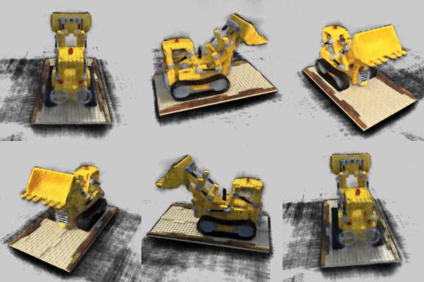
Bells and Whistles explanation: by simulating an infinitely large density at the end of a ray, we can convince the volumetric rendering principles into thinking there is a board of certain color at the end of the ray, and therefore, whenever the ray predicts not hitting any object or 3D point (originally resulting in black color), we convince it to think it has hit a white or gray board instead. The concrete changes only involve concatenating a large density value (say 100) and a targeted color different than black at the end of model predictions for densities and colors. However, this trick should only be done on evaluation, as we still want to train the model to think empty locations in scenes are dark.

Experiments

We conduct three main experiments:

[Part A] of the project asks us to train a two-dimensional neural field on one given and one self-defined image.
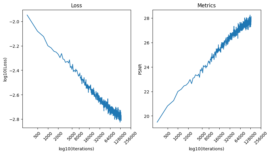
[Part B] of the project asks us to train and evaluate a three-dimensional neural field for a given scene, and reach a PSNR of $23$ at any iteration of our freedom.
[The Bells and Whistles] Change background of spherical rendering video.

Results

Part A: 2D Neural Field

We construct a 2D Neural Field on the following images:

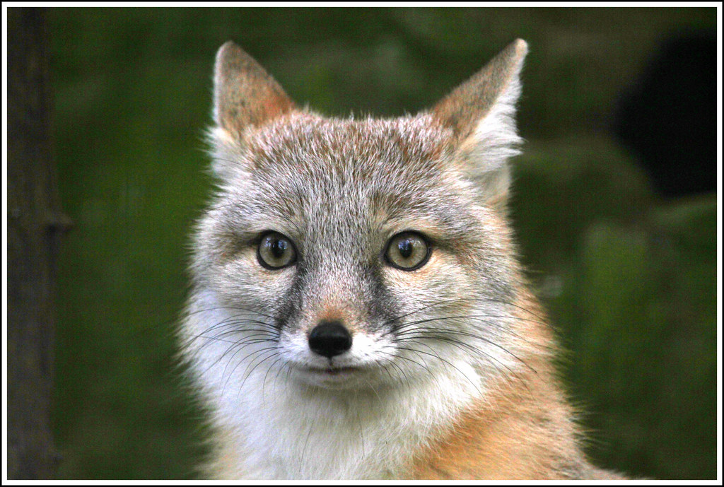
Here are the neural fields produced throughout training

Additionally, we assess the impact of two hyperparameters on the final result of these neural fields: the maximum frequency controller $L$ and the learning rate of the process.

The learning rate of the process had minimal influences:

The maximum frequency controller, on the other hand, had substantial influences. Particularly, with a larger $L$, the maximum permitted frequency in the image increases, and therefore allows for finer details int he image. Vice versa.

Part B and B&W: 3D Neural Field

To train a 2D neural field, we implement the architecture and volumetric rendering functions assigned in the manual, alongside other coordinate system transformations. We also select the following different hyperparameters from the spec, as the spec’s results are somewhat irreproducible:

A learning rate of $8e-4$ with per-epoch decay until $8e-5$.
Training for 100 epoch, where each epoch involves 400 gradient steps, each with a batch of 10,000 rays and 64 samples per ray.

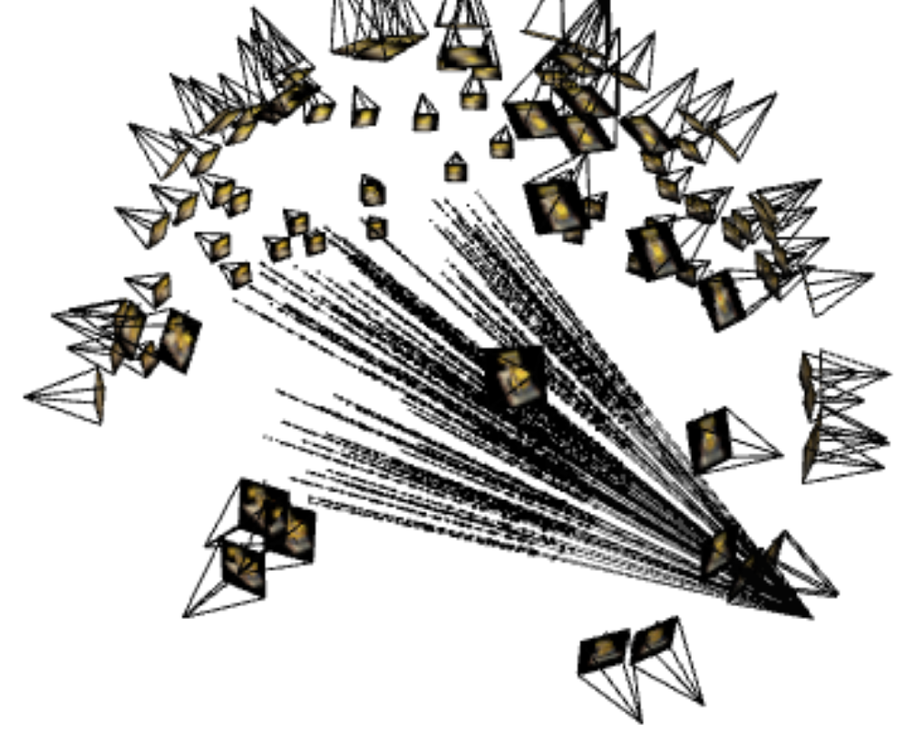
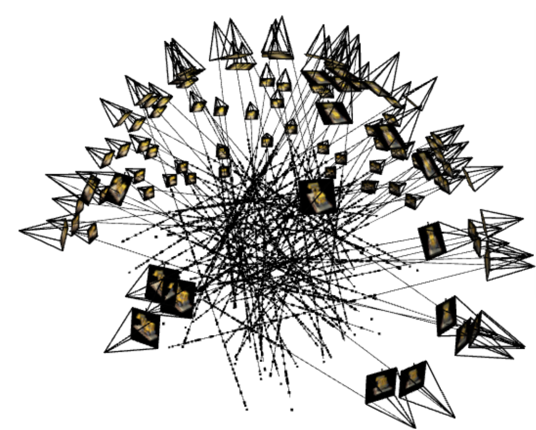
Here is a demonstration of the camera rays, the first image having all rays sampled from a single camera, and the second image having rays sampled across all 100 training cameras.

Here is the resulting training curve of our 3D neural field:

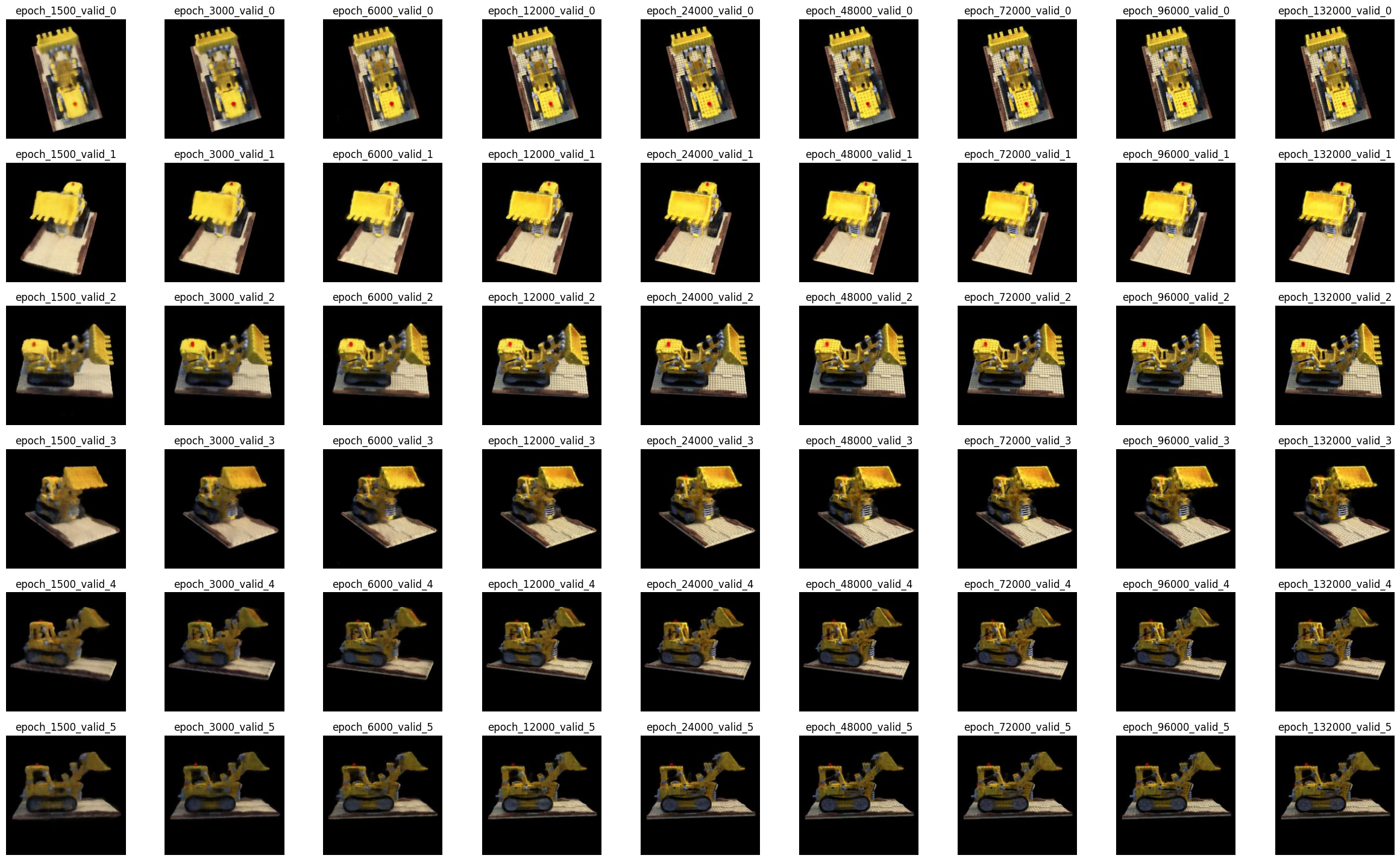
Here is how the validation set images change throughout the training process:

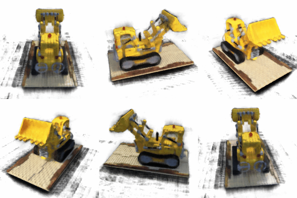
And here is a spherical rendering of our neural field on the test set cameras (transposed):

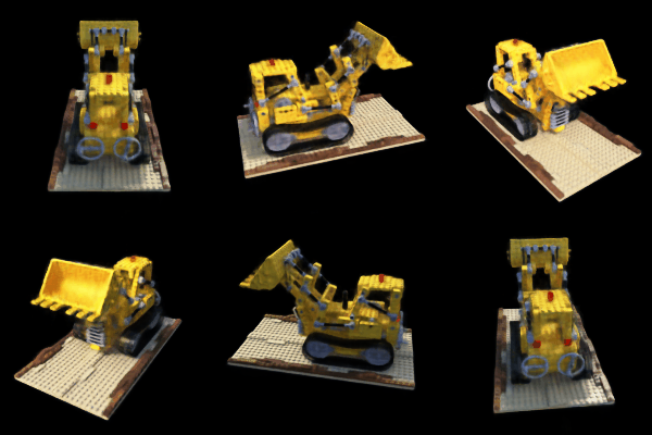
Its background color can be changed, but there will be dynamic dark noises as shadows are ill-defined in the scenes. The following GIFs result from 7000 gradient steps of training. The resulting dark signal can be thought of as an “overfitting” phenomenon where the model is overly convinced that empty scene locations must be dark.