[COMPSCI 180] Project 1: Color Channel Alignment
Published:
COMPSCI 180 Project 1 Writeup.
Introduction
Aligning color channels of an image is a prevalent problem for existing image files where the saved image in channels R, G, B are not well aligned. Specifically, an image might be offered as follows, where directly overlapping the three subfilms of the image results in an unideal picture. Several blog posts on the internet have addressed solutions to this matter, and witnessed successful results using classical methods with minimal linear algebra usage. In this blog post, we discuss the exercise of naive methods that can solve this problem, as well as the extent of limitation that these naive methods, extracted from suggestions in the homework instructions main page. Hopefully, the blog post is a quick write and a quick read, so I can go back and debug PPO afterwards.
Background
In this blog post, there are three major piece of knowledge that will be utilized throughout our methods introduced below: (1) the use of cosine similarity (not its extension, NCC), (2) a general method of exhaustive search for finding optimal displacement in smaller images, and (3) an image pyramid.
Cosine Similarity
Cosine similarity is widely used across many literature to compare vectorized representations, and recently largely applied onto computing the semantic similarity of embeddings. A vital application of cosine similarity may be found in attention mechanisms. Witnessing this success in cosine similarity, we will be comparing displaced imagges via cosine similarity.
An extension of cosine similarity, called Normalized Cross-Correlation (NCC), is a much superior choice. The metric is formulated as follows:
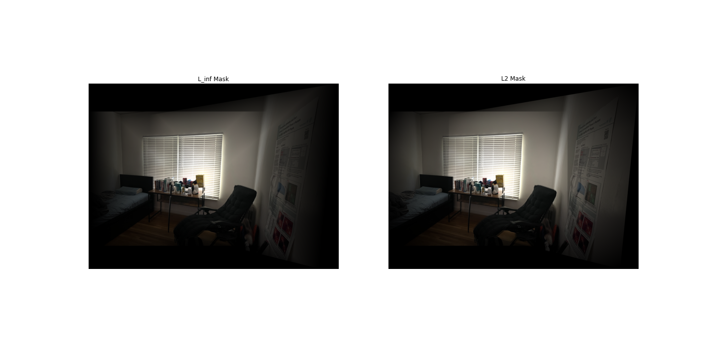
\[NCC(img_1, img_2) = cos(img_1 - \mu_{img_1}, img_2 - \mu_{img_2})\]This metric proves to be useful for most images except emir, while picking the right hyperparameters for a search process with the cosine metric performs a more consistent alignment across images. Therefore, in this post, we only use cosine similarity as the metric for comparing images.
Optimal Displacement Search in Small Images
To find an optimal displacement (two-dimensions) for small images, we can first target a search-space (say, from offsetting an image with -15 pixels to 15 pixels), and try each two-dimensional vector within the range ${-15, \dots, 15} \times {-15, \dots, 15}$. This means the search-space scales quadratically with the amount of offsets we want to investigate per dimension. In such sense, this method essentially solves the following optimization problem via exhaustive search:
\[\max_{x \in [-15, 15], y \in [-15, 15]} \cos({\rm offset}(img_1, x, y), img_2)\]Here, the ${\rm offset}$ function is implemented as a img1.roll(x, y, axis=(0, 1)) call. A cropping approach was attempted in the middle of the project, but replaced with the above option for solution of better quality.
Image Pyramid
While the above method is proven effective on smaller images (specifically, with each dimensions being less than 400 pixels), it will take a large amount of time on larger images. Therefore, a school of method employs the approach of first solving the displacement finding problem on a small, downsampled version of the image, then adjusting its estimate of the optimal displacement as the base problem is solved and the image is upsampled. Particularly, the method can be phrased as an iterative procedure with the following steps:
- Downsample the image until a base problem size, in our setting when either of the image’s dimension is less than 400 pixels.
- Solve the optimal displacement search problem on the image, checking offsets in $[-15, 15]$.
- Upscale the displaced image by the original downsample factor.
- Solve the optimal displacement search problem on the upscaled image, with a smaller problem size. In our case, we check offsets $[-1, 1]$.
- Go back to Step 3 until the image is cannot be further upscaled. This is a U-shaped process, where we begin from the original size of the image onto the first, then second, gradually the kth layer of image pyramid where the image is downscaled to the base problem size, then recede along the pyramid to return to the originally-sized image where a displacement is found.
Recursively, we may phrase the final found displacement with the following mathematical expression. Suppose the $(n-1)^{th}$ downscaled image finds a local displacement of $(x_{n-1}, y_{n-1})$, and the local displacement found on the nth downscaled displaced image is $(x_{local, n}, y_{local, n})$, then the true displacement found at the nth layer of this process would be $\left((x_{n-1} / f_{downscale}) + x_{local, n}, (y_{n-1} / f_{downscale}) + y_{local, n}\right)$.
Methods and Results
Optimal Displacement Search on Low-Res Images via Single-Scale Approach
The overall flow of our solution is as illustrated in the following figure:
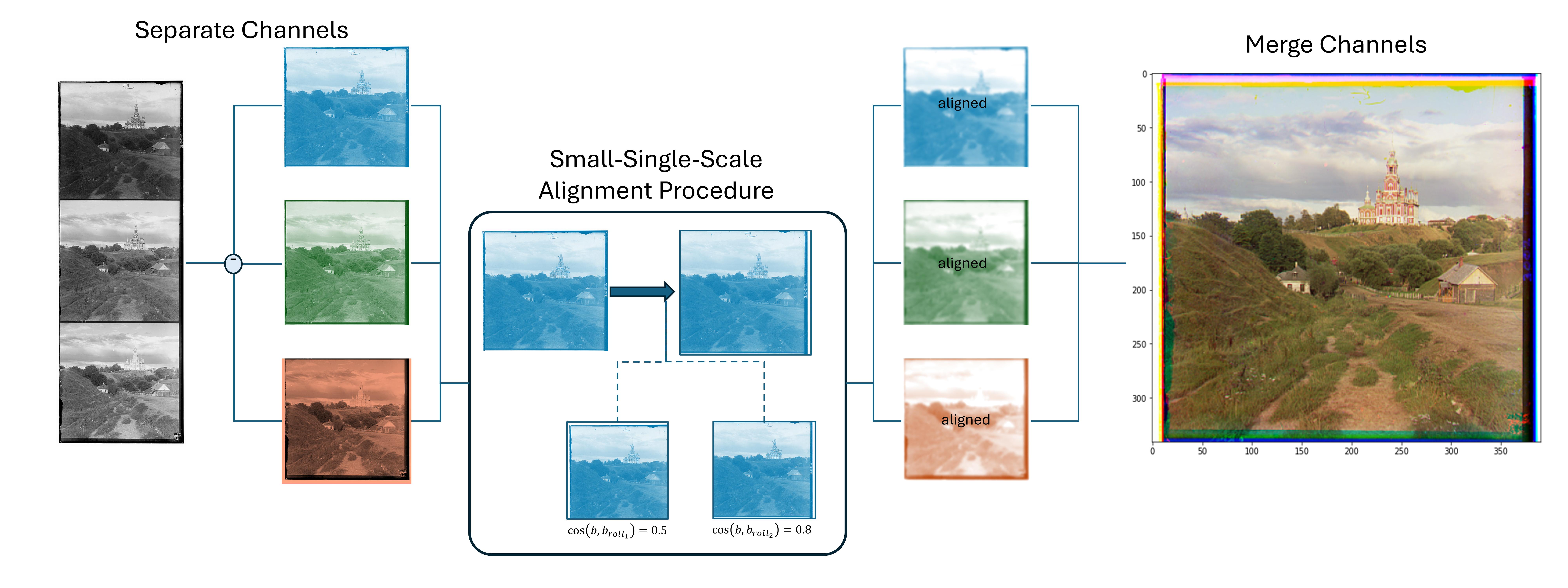
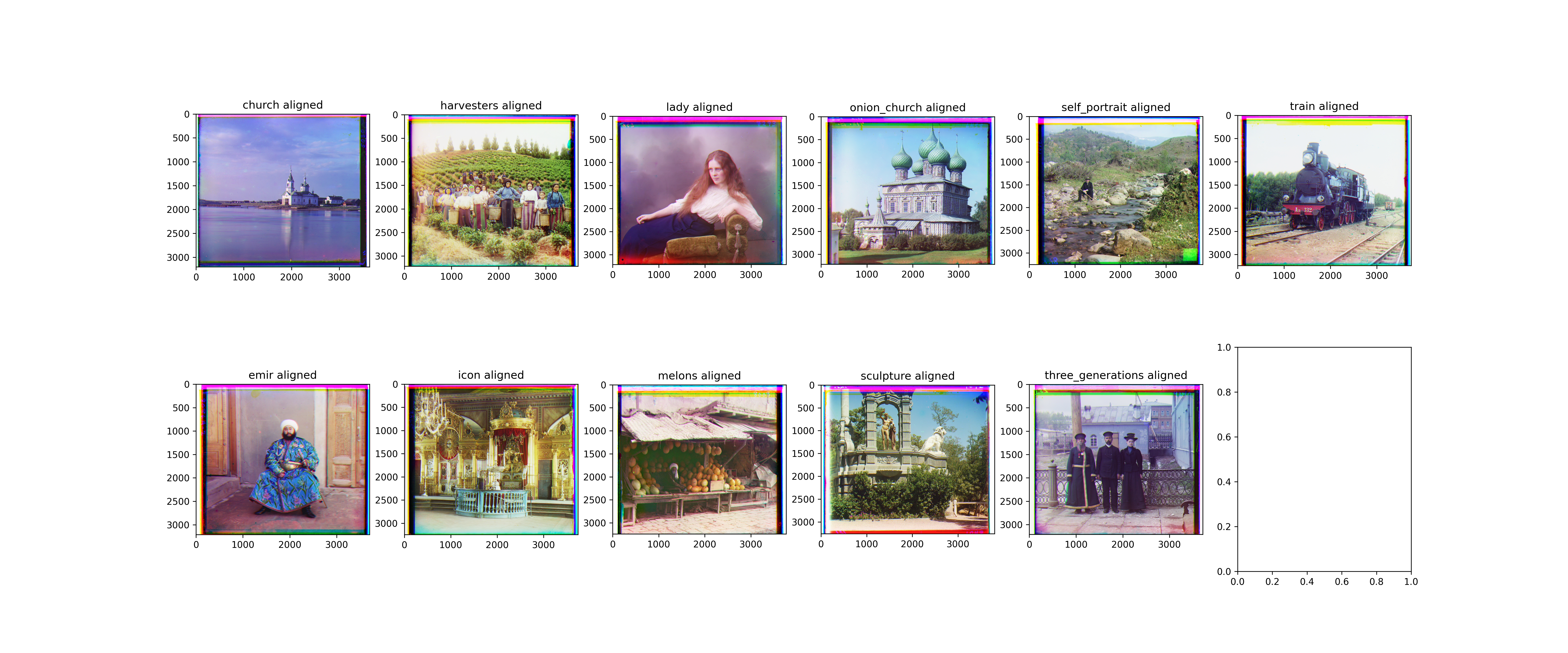
First, provided a .jpg file containing all three channels of the image separately, we separate the channels of the image by slicing it into three parts with equivalent heights. Then, we crop the edges of the image away to avoid noisy information by taking $10\%$ of each dimension’s end away. Next, we perform the small single-scale alignment procedure over a problem space of $[-15, 15] \times [-15, 15]$ pixels as stated in our Background section. Upon finding the appropriate displacements, we roll the images according to the found solution to recreate the original image.
A survey of the provided image’s outcomes can be seen as follows:
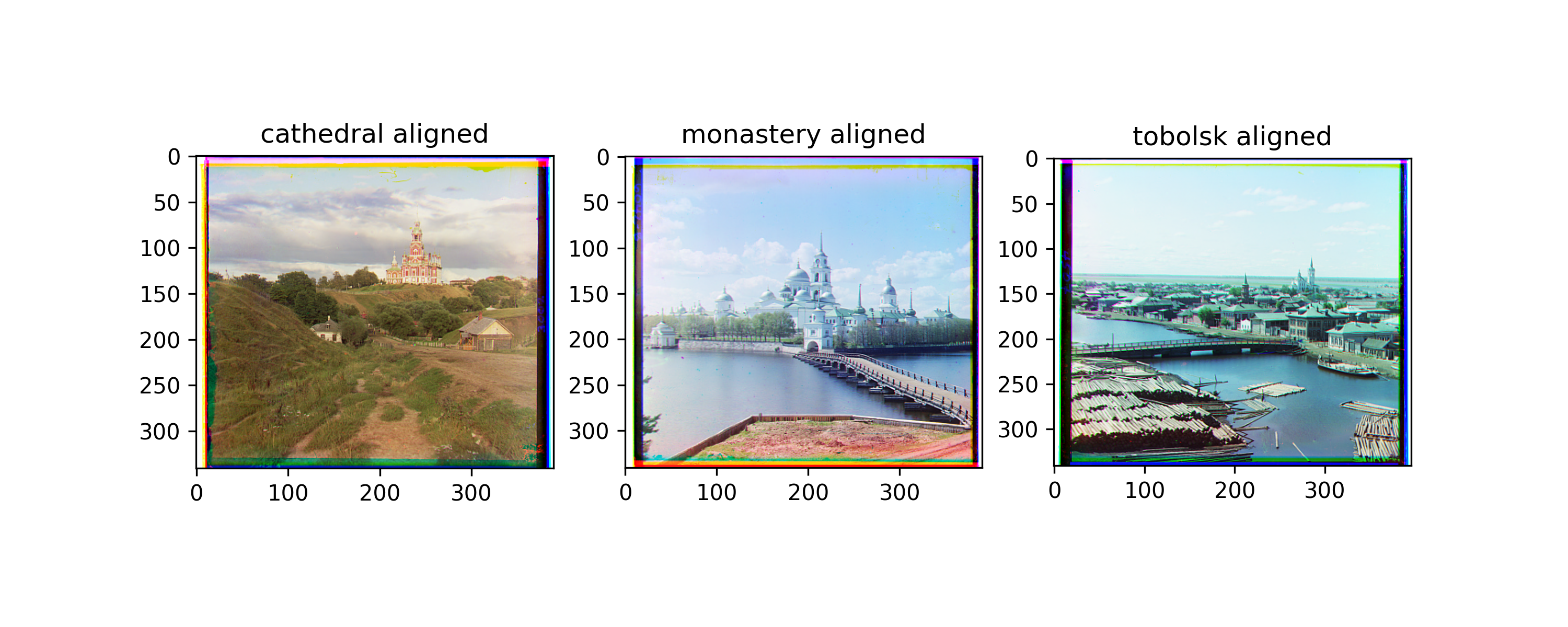
Image Pyramid-Empowered Multi-Scale Approach
The overall flow of our solution is as illustrated in the following figure:
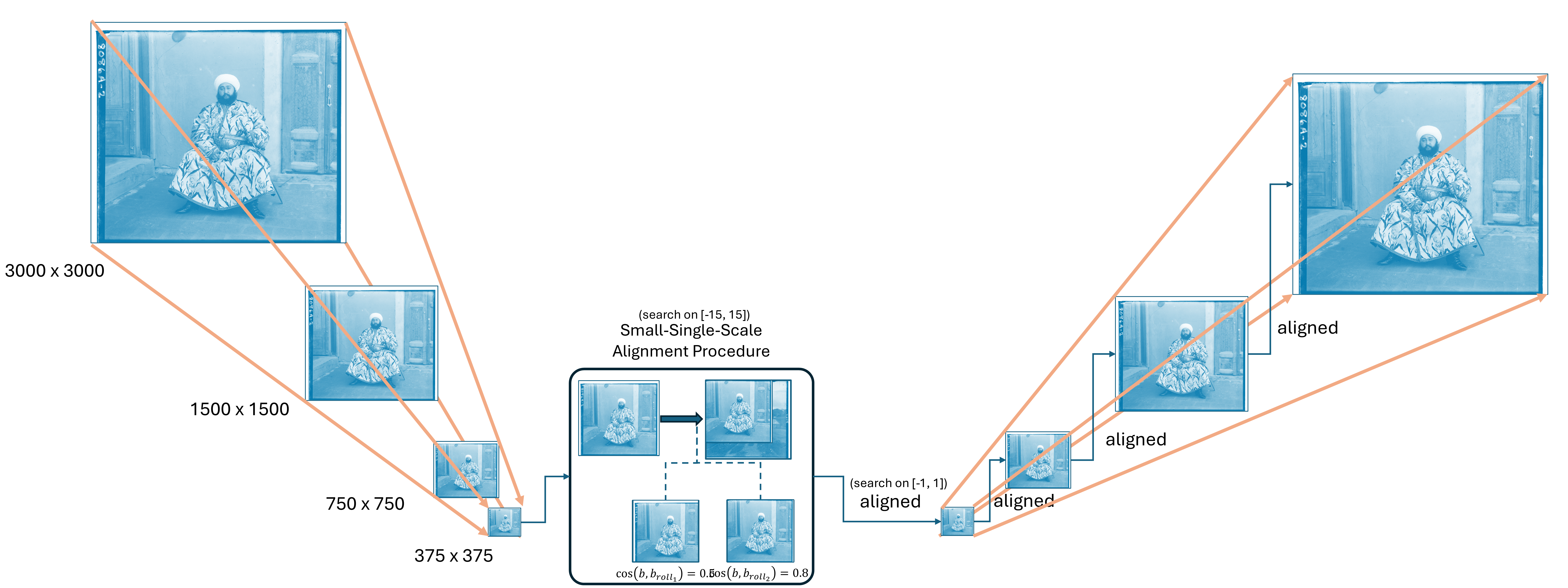
First, we separate the provided .tif image file into three subparts of equivalent height as shown in the single-scale approach. Then, we follow the image pyramid approach with a problem size of $[-20, 20] \times [-20, 20]$ pixels in the base problem, and $[-1, 1] \times [-1, 1]$ pixels for subsequent upscaled layers. The downscaling factor is $0.5$. Note that, an empirical test has been performed for downscaling factors across $0.25$ to $0.95$, and the chosen value performs most consistently across the desired set of images. The results are exhibited as follows:
Then, here is a table of found displacements that produces the following images:
| Name | Red Displacement | Green Displacement |
|---|---|---|
| Cathedral* | (12, 3) | (5, 2) |
| Monastery* | (3, 2) | (-3, 2) |
| Tobolsk* | (6, 3) | (3, 3) |
| Church** | (66, -7) | (33, 7) |
| Emir** | (108, 66) | (58, 33) |
| Harvesters** | (134, 24) | (66, 24) |
| Icon** | (100, 33) | (49, 24) |
| Lady** | (125, 9) | (58, 16) |
| Melons** | (177, 16) | (92, 15) |
| Onion Church** | (117, 41) | (58, 33) |
| Sculpture** | (151, -25) | (41, -8) |
| Self Portrait** | (177, 41) | (84, 33) |
| Three Generations** | (117, 16) | (58, 24) |
| Train** | (100, 41) | (49, 16) |
*: Obtained via single-scale; **: Obtained via multi-scale.
Discussion and Conclusion
In this blog post, we successfully replicated preliminary methods for color channel alignment. I will now go back and debug PPO :’)