COMPSCI 180 Project 2 Writeup

*Note: Although I use the pronoun ``we’’ in this writeup, this is simply becuase I have been converted beyond the past innocence of using “I” at any academic setting due to a recent intoxication of arXiv products. Meanwhile, please bear with the lack of theoretic figures as opposed to in the last post, where some illustrations are provided to explain concepts.

Introduction

In this assignment, we explore a fundamental aspect of signal processing and computer vision– filters. Filters are mathematical objects that allow for the removal of components with certain frequencies within a signal. They are useful when we need to remove a high frequency component of the signal. For example, when a vocal recording has too much high-pitched noise, one can use a low-pass filter to permit all of the low-frequency components in our recording, effectivly excluding the high-frequency noises we mentioned before.

In images, this technique is applied across several purposes, and today we dive mostly into the construction of images and edge detection via use of filters coupled with many familiar mathematical notions: derivatives, gaussian distributions, and convolution. In this writeup, we detail the work we have done across several tasks assigned throughout the assignment.

Preliminaries

This section outlines the preliminary methodologies used within this assignment to fulfill numerous objectives, containing all methodological descriptions of the images’ creation. Experimental details, such as the use of hyperparameter and particular reflections on the product, are detailed in later sections. For external readers, this section serves as an overview and review of techniques; for graders, this section serves as a proof of the writer’s understanding of concepts for relevant grading items. Last but not least, for the writer, this section serves as a trial towards the completion of assignment and a finally coming period of freedom upon the writing’s accomplishment.

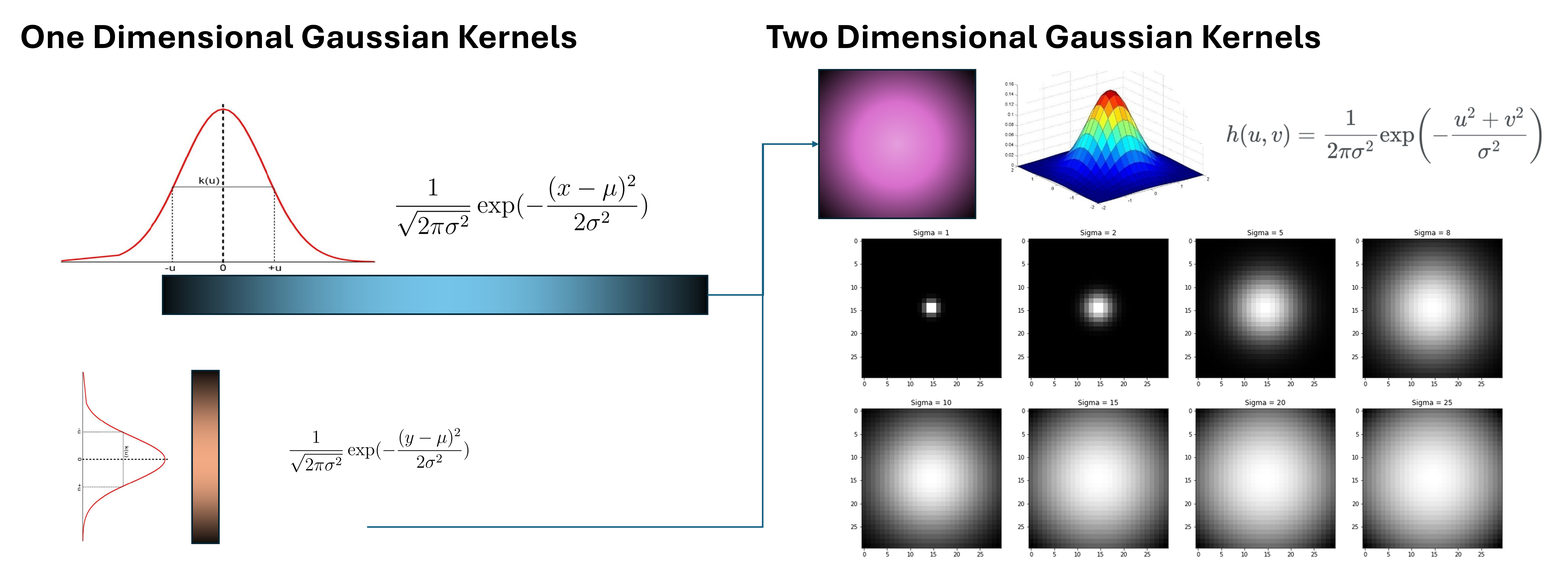
Gaussian Kernels

A kernel is a matrix that we can perform cross-correlation with an image on. So, particualrly, a Gaussian kernel is a kernel that can be used to perform cross-correlation, but with its values across the kernel’s matrix distributed based on the Gaussian distribution. That is, following a specific density function, values at the center of the matrix enjoys a much higher weight than those at the edge of the matrix. A demonstration of Gaussian kernels with width $30$ across various standard deviation value selections follows:

Particularly, it follows the following density function:

where $\sigma^2$ serves as a hyperparameter for smoothing– the larger $\sigma$ becomes, the more smoothing involved in the process. Usually, we choose a kernel width of $6 \sigma$. Unless noted otherwise, we use this standard for kernel width throughout the post.

This format allows for outcomes of cross-correlations to be a weighted average of some block of pixels, where the weights are normalized as they are individual kernel values coming from the Gaussian distribution, which should have an area under curve of $1$ as a density function. In such manner, applying a Gaussian kernel onto a picture is essentially equivalent to creating a smoothed version of the image, which preserves the low-frequency elements of an image. In such manner, as the low-frequency images are stored, we call this act of application a “low-pass filter”.

Image Derivative

For an image as a discrete function $f(x, y)$, recall that the derivative of a continuous function could be computed as:

which brings us to a discrete equivalent:

or potentially,

These computations can in fact be presented as convolutions. Particularly, the primary derivative comes with the filter $\begin{bmatrix} -1 & 1 \end{bmatrix}$, while for the latter $\begin{bmatrix} -1 & 0 & 1 \end{bmatrix}$.

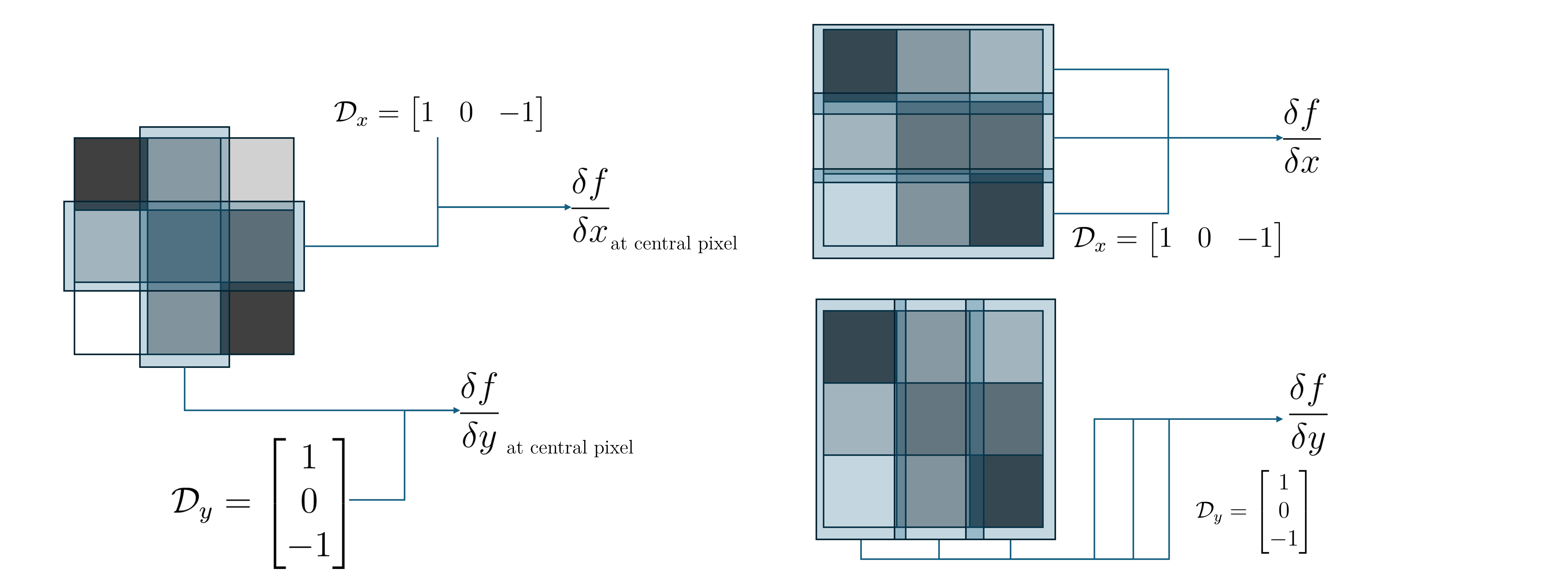
Meanwhile, we can simiarly propose the formulation of an image gradient:

The edge of the image can even be found from the gradient magnitude:

The direction of the gradient can also indicate the direction of the lighting (although it also hallucinates some structure):

Convolution and Filters: A Signal-listic view of Images

Convolution is a mathematical operation defined as follows.

Let $F$ be the image, $H$ be the kernel, and $G$ be the result of this operation. Then,

Otherwise denoted as: $ G = H \star F $ It is commutative and associative. Therefore, all of the following expressions hold:

At the edge of an image, one can choose to partially apply the kernel or not. Different libraries made different calls. In this project, we choose to preserve the original image size, and make convolutions at the edge of an image based on this policy.

Notbaly, while a Gaussian kernel removes high-frequency components from the image, working as a low-pass filter, convolution of Gaussian kernels is another Gaussian kernel. That is, for a Guassian kernel of width $\sigma$, its self-convolution has width $\sigma\sqrt{2}$.

The application of convolution is diverse. Without addressing the theoretical formulations of it, here is a list of operations performed in our assignment:

• Vectorizable Image Gradient Calculation: Provided that the derivative of an image at a point is its surrounding block of gradients multiplied by the $\frac{\delta f}{\delta x}$ operator (and $\frac{\delta f}{\delta y}$ alike), we may apply a convolution of these operators as masks/filters onto our image to obtain an image gradient in the operator’s direction.
• Gaussian Low-Pass Filter: As mentioned in prior section, the Gaussian kernel can act as a low-pass filter once applied via convolution onto the image.

My Perspective of Your Image

There are two popular formulations for the composition of an image: (1) a pixel-based function and (2) a mathematical entity in a signal-basis space.

A pixel-based function view of the image maintains that one may imagine an image as some sort of function:

where $r(x, y)$, $g(x, y)$, and $b(x, y)$ are the red, green, and blue intensities at the point $(x, y)$.

The signal-istic view of image, on the other hand, originates from empirical results like Campbell-Robson contrast sensitivity curve, which converge at the idea that humans are sensitive to different frequencies at different orders. In such case, formulating the image as a sum of many waves should enable us to decompose the image more efficiently along the human perception space (and generally, a biological perception space).

Each signal contains a fundamental building block of:

as a possible member of the ``signal basis’’. And, it is hypothesized that with enough of these blocks added, we can obtain any signal $f(x)$. Note that, however, each of the building block possesses three degrees of freedom: $A$ (amplitude), $\omega$ (frequency), and $\phi$ (phase). Particularly, the frequency constructs and encodes the fine-ness of this signal. Fourier Transform is an oepration that manages to separate one image into several building blocks (as well as obtaining their coefficients).

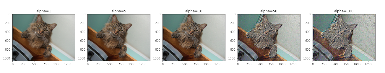
Application: the Unsharpen Mask Filter

The signal-istic view of an image introduces us to the idea that an image has a low-frequency component and a high-frequency component. High-frequency components refer to the finer details of an image where change occurs rapidly, such as the edges of an image; low-frequency components refer to the coarser details of an image, such as the general silhouette of a portrait. We have learned that the Gaussian filter helps us extract the low-frequency component of an image. Then, since the image is a sum of low-frequency and high-frequency signals, the signal-istic view suggests that subtracting the low-frequency components of an image away ought to provide us only the high-frequency signals: the sharp edges of an image and the subjects within it. Therefore, we can reinforce the edges of an image by adding the high-frequency signals: $f - f \star g$ onto the original image $f$.

However, it may occur that the high-frequency component of the image does not have a large enough magnitude, so we may want to add a scalar multiple of it rather than its original, forming the computation:

The mathematical properties of convolution allow us to summarize this sharpening action, called an unsharpen mask filter, as an operation involving one single filter:

Gaussian and Laplacian Pyramids

In the last assignment, we have worked with a naive image pyramid that downscales images and upscales them back, allowing for a recursive problem-solving structure:

In a Gaussian pyramid, we apply this structure by attaching a Gaussian filter to the construction of each layer downwards, such that each subsequent layer experiences a low-pass filter and is also downscaled. Computation with a prior layer, which contains an image two-times larger, involves the rescaling of a smaller layer. The Gaussian pyramid therefore contains images of differing low-pass results, which selects lower and lower frequency components. Consequently, subtracting each consecutive layer grants us a range of frequency components between those consecutive layers, essentially creating what we call a bandpass filter (bandpass means middle-pass, as opposed to low-pass or high-pass).

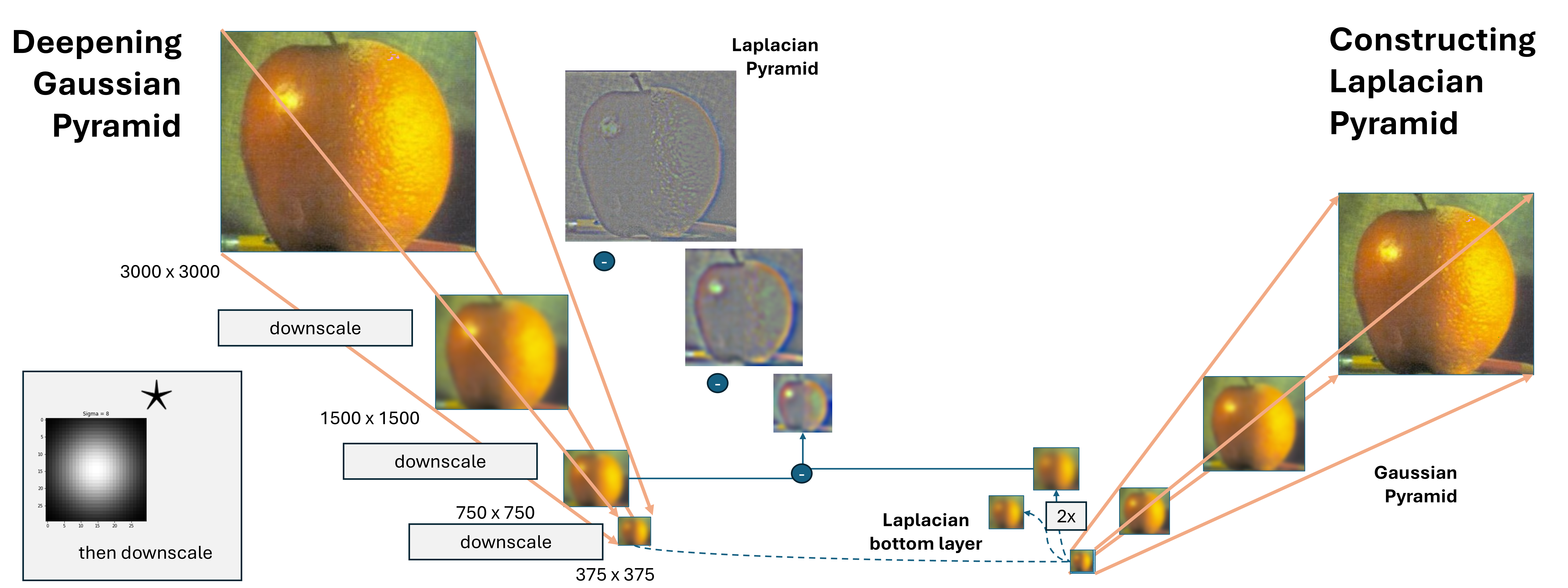
Therefore, based on the above theory, we may construct a modified framework called the Laplacian pyramid, where each layer of the Laplacian pyramid is the difference of some respective difference of Gaussian pyramid’s consecutive layers. By propety, Laplacian pyramids have one layer less than Gaussian pyramids, so the final layer of Laplacian pyramids are formualted to be the last layer of Gaussian pyramid.

To summarize, in a Guassian pyramid, there is a cascading of several low-pass filters, which splits the signals by bands in the filter. To obtain a bandpass pyramid rather than a low-pass pyramid, we can subtract each layer and an upsampled version of its previous layer. This variation, which is called a Laplacian pyramid, performs Laplacian filters which accept higher frequency waves.

On the other hand, a Laplacian pyramid then contains images with only the bandpass frequencies. Usually, we find local structures to be stored in the Laplacian pyramid, which becomes coarser as we traverse into deeper layers of the pyramid. And because of the Laplacian pyramid’s property as a consecutive difference, as we add all the images in a Laplacian pyramid and the lowest frequency picture in the Gaussian pyramid, we can recover the original image.

For external readers, please refer to this slidework from COMPSCI 180 of UC Berkeley for brilliantly illustrated intuitions and insights.

Fun with Filters

Overview of Methodology

In this problem, we consider the cameraman image:

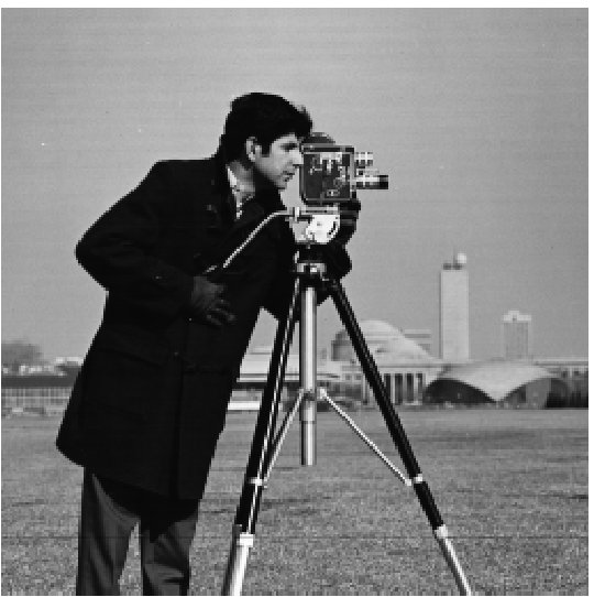
and we want to extract the edges of this image. Following the theoretic insights described in the previous section, two natural solutions stand: (1) using a very-high-pass filter, or (2) using an image gradient magnitude image. In this problem, we consider the latter.

Particualrly, we experiment on three different methods: (1) naively using the image gradient magnitude image, (2) applying a Gaussian filter first, then applying the image gradient magnitude treatment, and (3) applying the convolution of Gaussian filter and image derivative operators, then obtaining the image gradient magnitude.

Notably, by the mathematical property of convolution, methods (2) and (3) are theoretic equivalents. Therefore, a portion of the work below will also concern the equivalence of outcomes between methods (2) and (3), beyond the improvement that they can provide beyond (1) in reducing high-frequency noises coming from the grassland background of cameraman.png.

Naive Image Gradient Magnitude

Via methods described in the theory section, we arrive at the following picture:

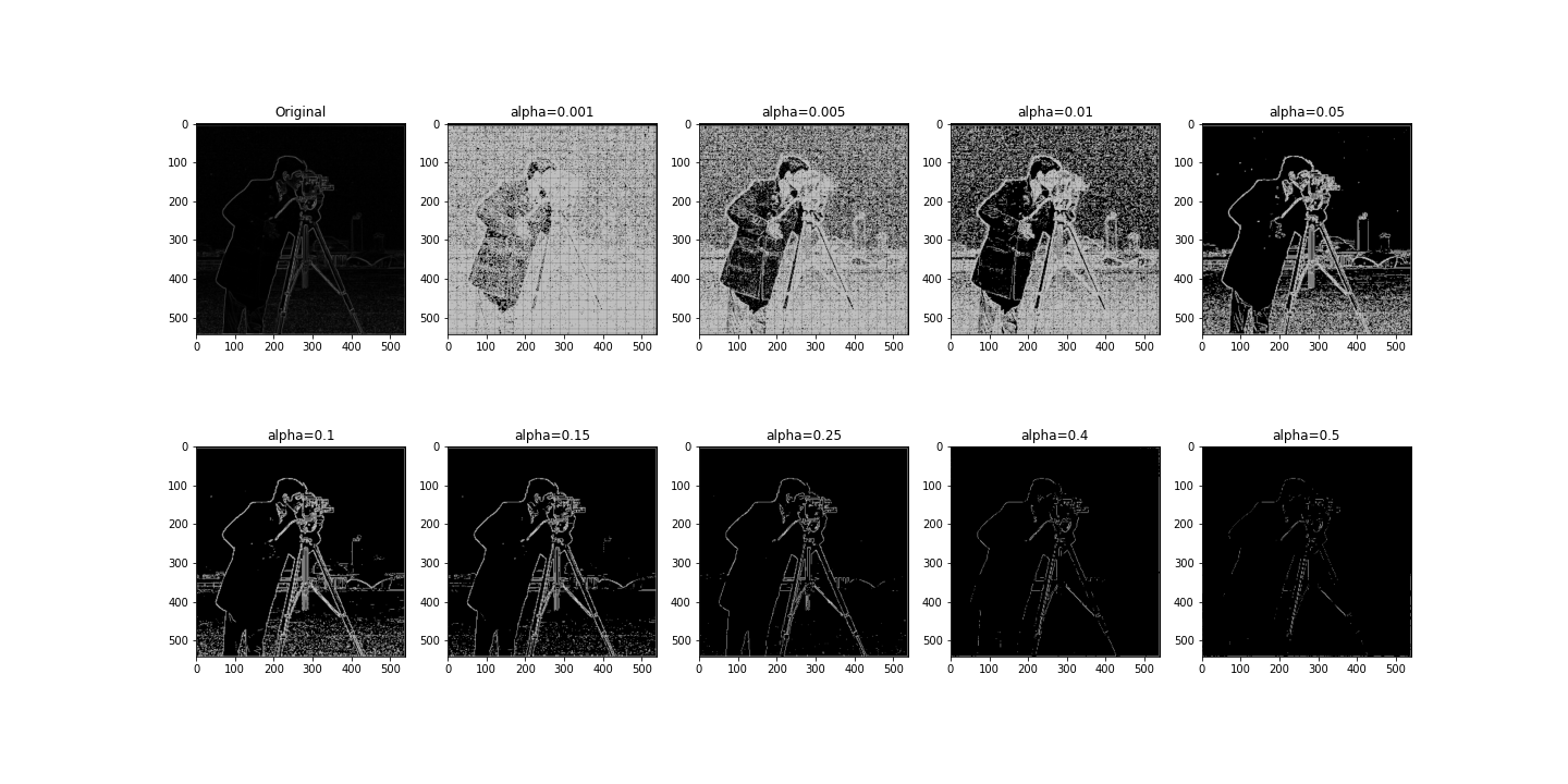
Here, each subplot concerns a specific cutoff of the image. Particularly, the shown $f_{clip}$ of image gradient magnitude image $f$ is clipped such that all values above the specified $\alpha$ has pixel-values set to 1, and otherwise 0. The original pixel values are shown in the subplot called Original. Empirically, we see that the $\alpha$ treatment helps to make the elicited result more concrete, but also observe the accompanying noises it can bring upon. Therefore, we choose to first smooth out the noises by applying a low-pass filter (enacted as a Gaussian kernel and convolution), then applying our current technique.

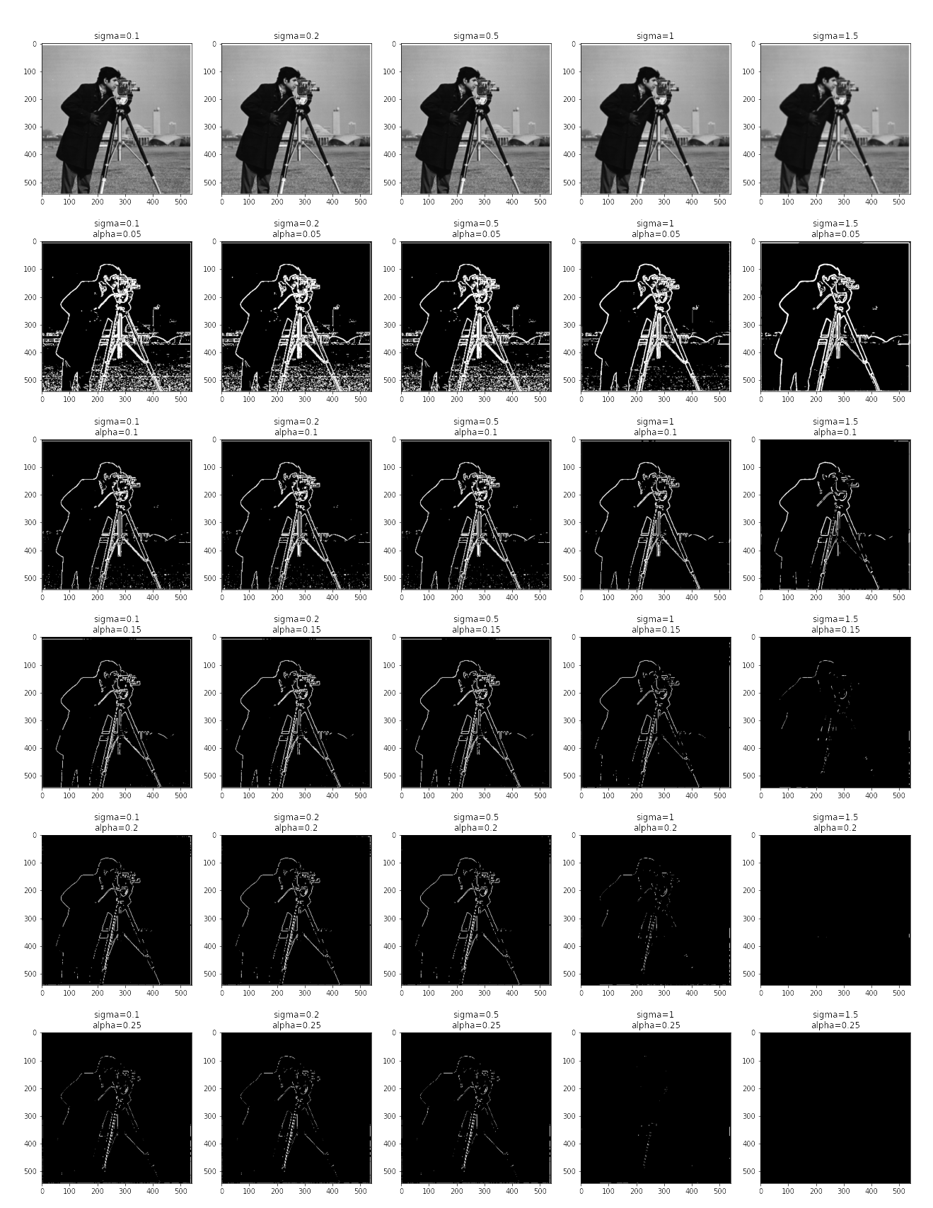
Gaussian Filters Goes Brrrr

Here, the Gaussian filters are created as an outer product of two 1-dimensional Gaussian filters, each with a width of 30 and a standard deviation denoted upon the figure.

Method (2)’s outcome is as attached below:

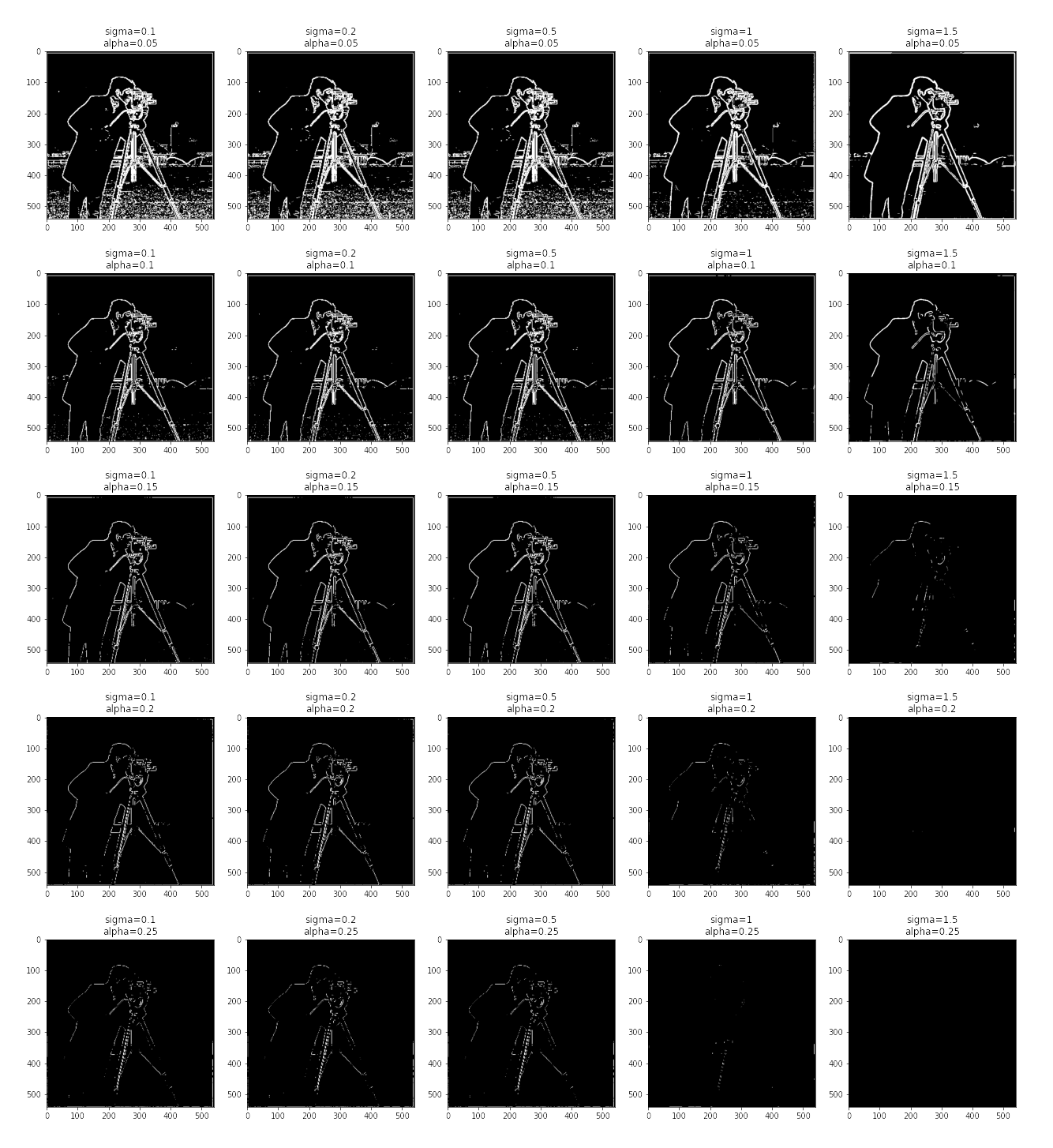
Meanwhile, method (3)’s outcome is as attached below:

and its filters are:

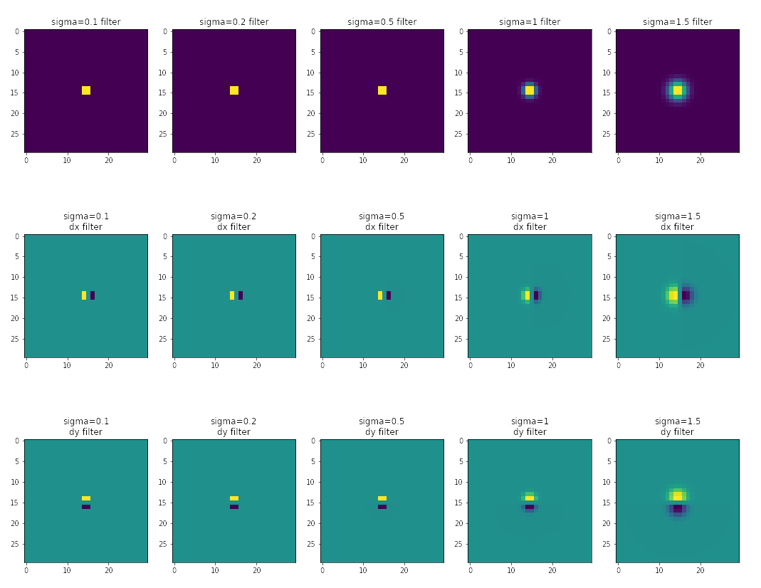
Here, we witness an empirical similarity of results in methods (2) and (3), and also note the significant improvement of edges’ clarity and noise removal at the rightmost column of methods (2) compared to the best outcome in method (1). Therefore, all qualities of the assignment’s problem are satisfied.

Fun with Frequencies: Image Sharpening

Overview of Methodology

We directly apply the aforementioned unsharpened mask filter in the preliminaries section on every investigated image.

Sharpening Blunt Images

Let’s look at the proposed mask’s effect on some soft/blurry images:

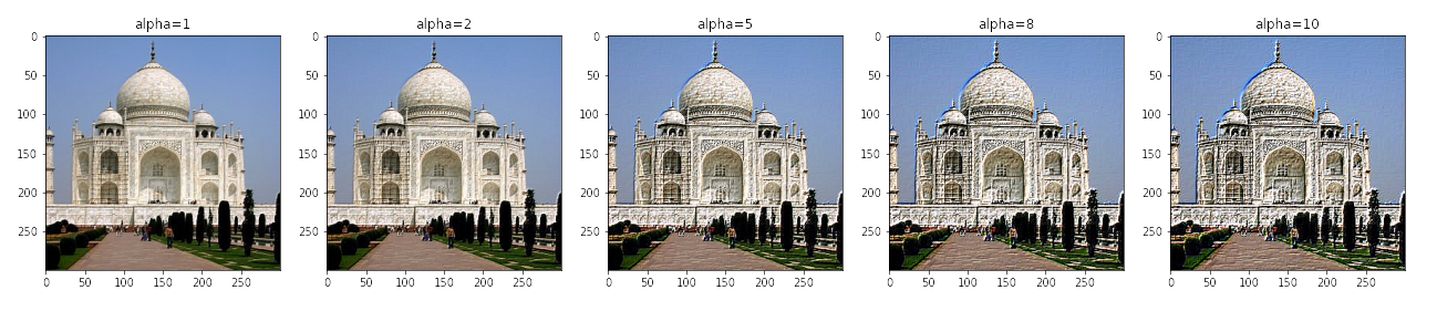
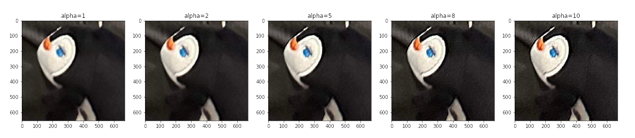
Across all alphas, we see a reinforcement of higher-frequency details in the image. This trend persists in sharper images:

Fun with Frequencies: Hybrid Images

Overview of Methodology

Hybrid images are (possibly cursed) pictures that occur to appear as two different images at the same time. This occurs by mixing the high-frequency aspects of one image and the low-frequency aspects of another, which can cause the image to look differently across different viewing distances. Below, we demonstrate such operation with the example of a Derek-Nutmeg (catboy, or Nutrek, if not Dermeg, but preferrably catboy).

The procedure of creating a hybrid image is outlined as follows:

1. Use the provided code to align the two images that will be mixed together, forming two images with the same dimension.
2. Extract the low-frequency aspects of the far-viewable image, and the high-frequency of near-viewable. In the case of a catboy, boy is far-view and cat is near-view.
3. Average the two images together, and hold the image either absurdly close or far to spot a cat and a boy in the catboy.

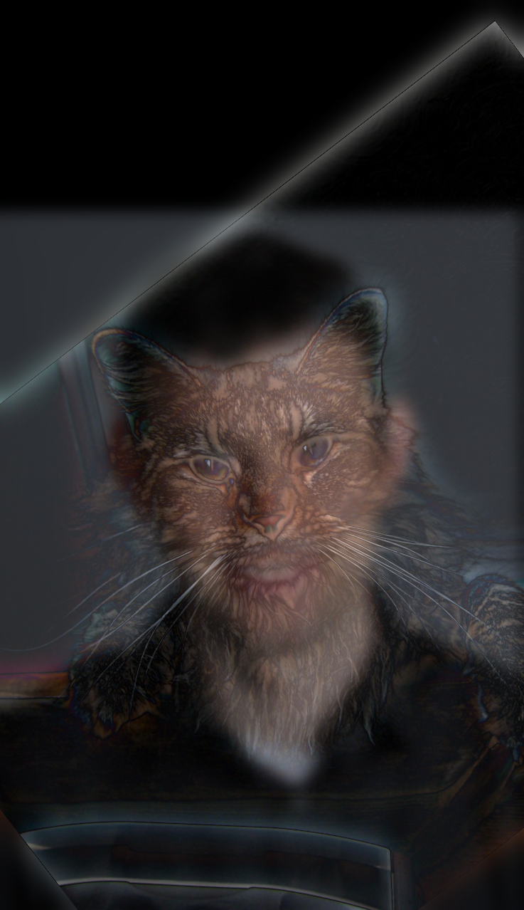
catboy

Let us first discuss the catboy.

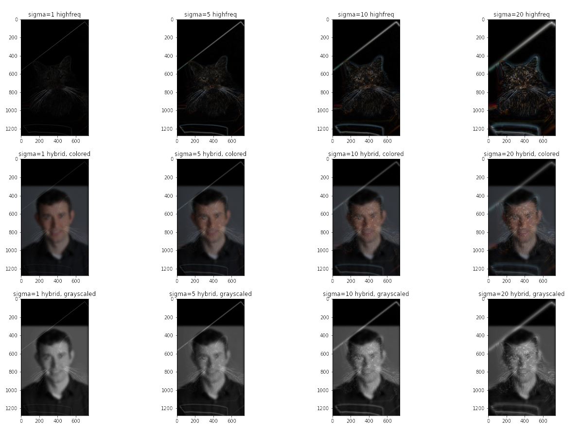
We may examine our catboy closer:

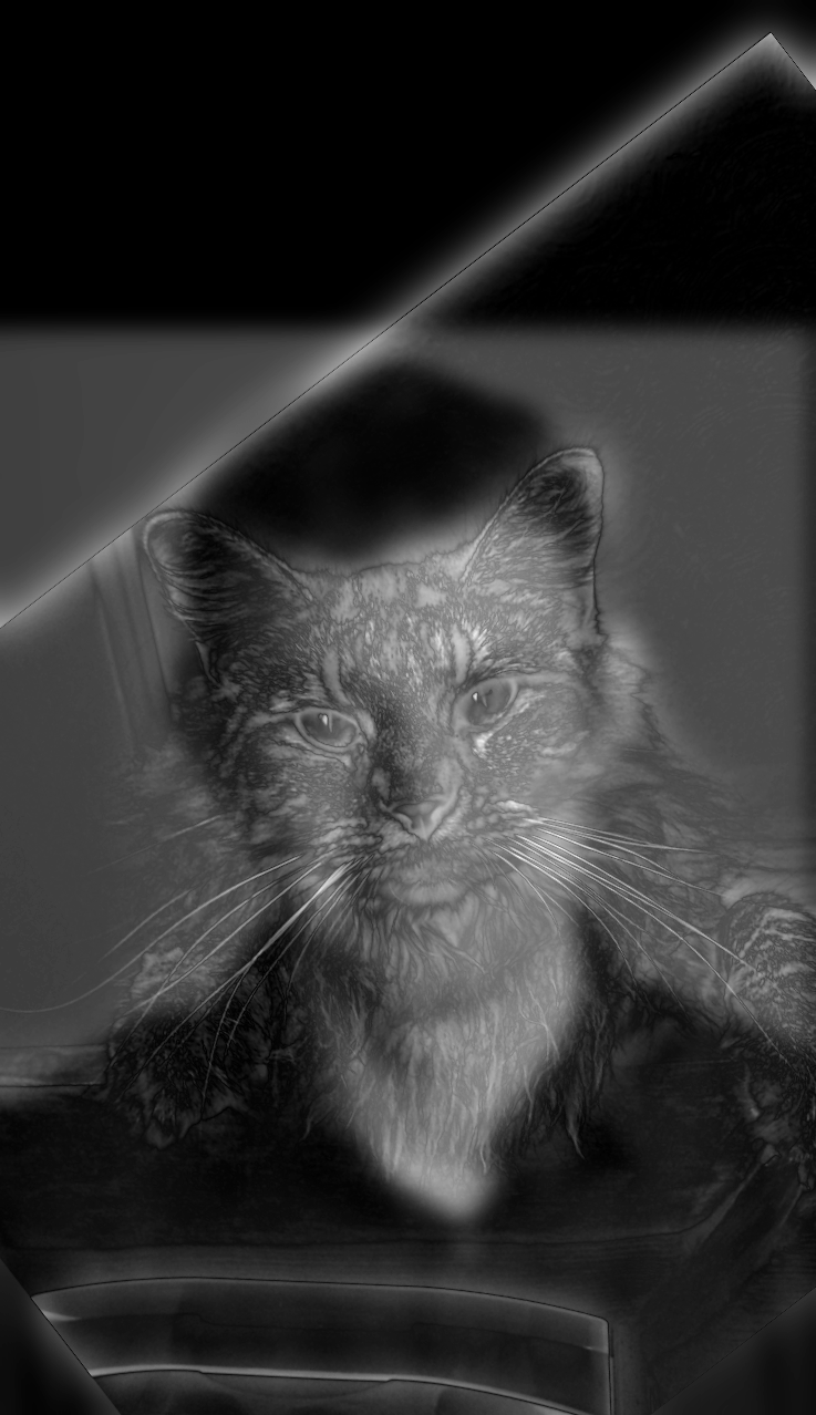
To prove the theoretic assumptions postulated above, let us look at the frequency maps of low-frequeney Derek variant and high-frequency Nutmeg variant, attached below in the order they are addressed above:

In this manner, we indeed observe that high frequency variant of nutmeg entertains a wide range of higher frequencies, while the low frequency variant of the Derek image entertains mostly low frequencies except some beam of higher frequencies.

Notably, low-frequency components are better off colored than not, as high-frequency components being colored will make them more dominant at a further distance.

Failure cases

There are several failure cases we can discuss, but I’d look at this one: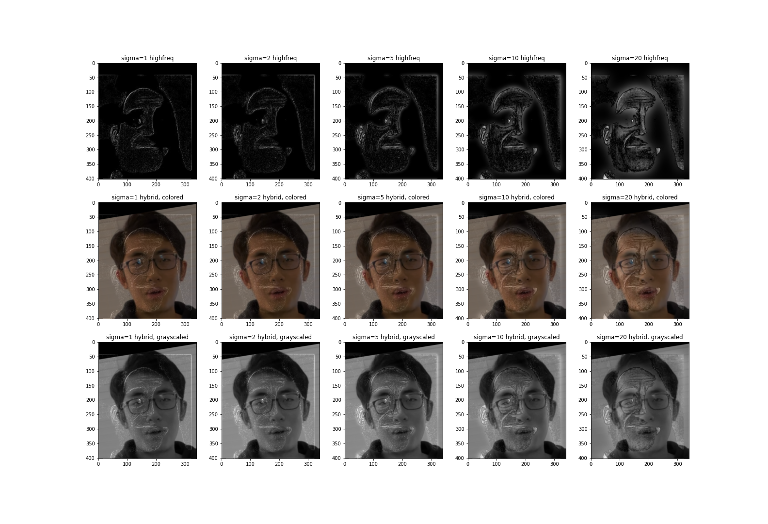

In this one, it didn’t work because the high-frequency picture of the canny face (captured at top row of above plot) is hard to elicit in clarity, and the two images are also hardly align-able.

Exercises that were Left to The Writer, but now to The Reader

With the above techniques, let us compose two more hybrid images.

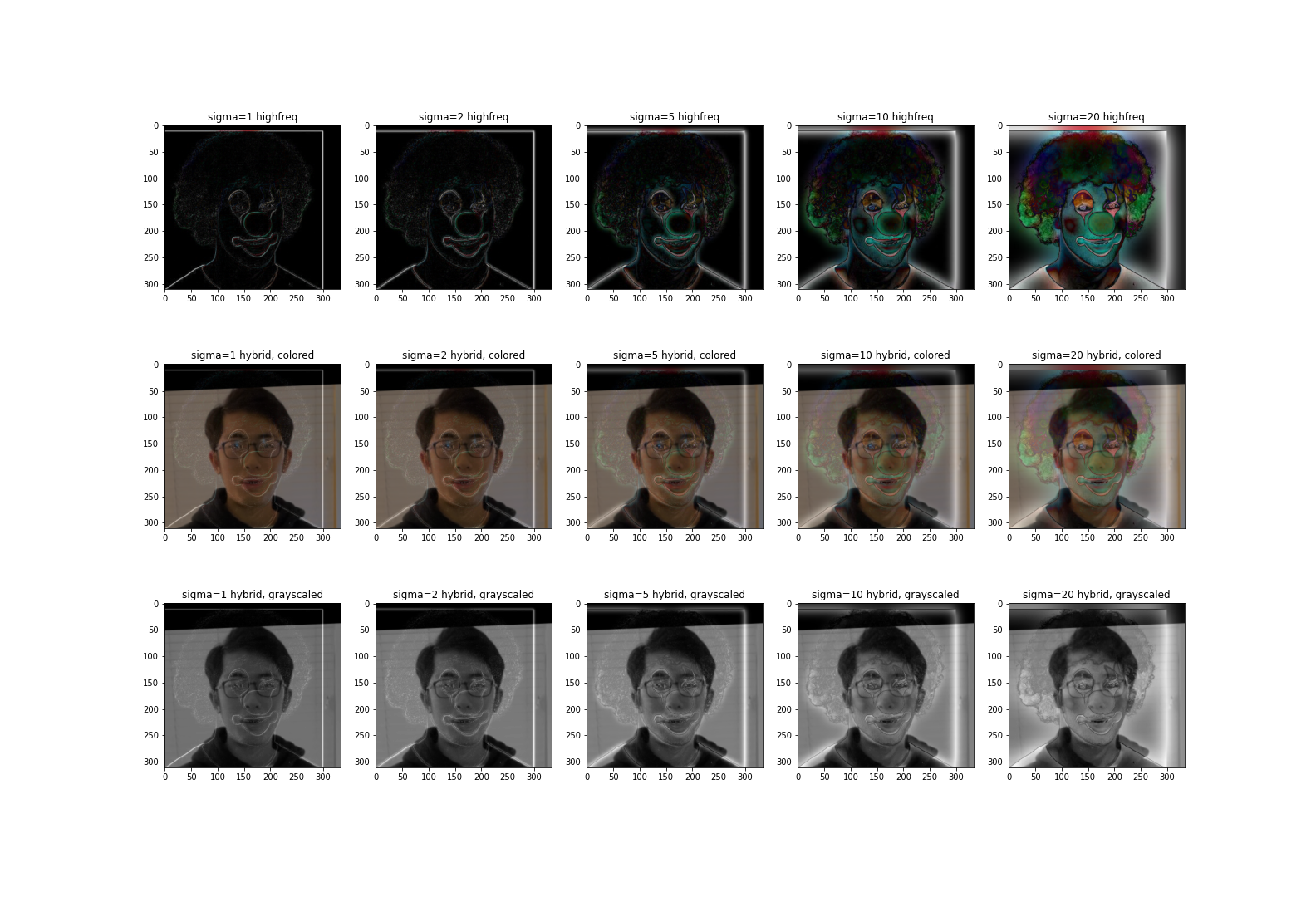Choose a coefficient set of your preference from above to form your favorite Clown-rus. Qualitatively, then, Cyrus’s picture is left more adapted to the clown picture rather than the uncanny picture in the prior subsection.

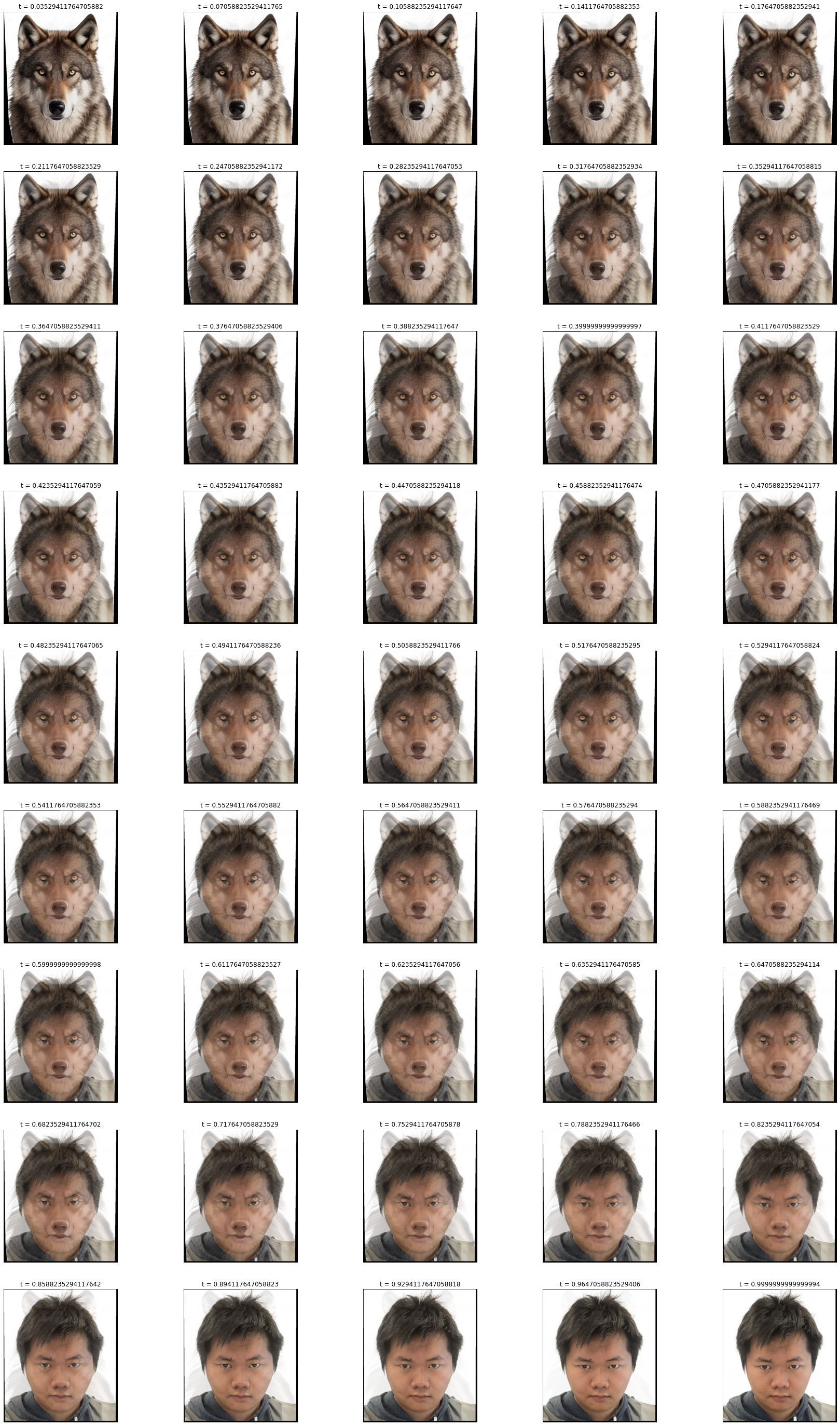
On the other hand, let us picturize our deer Ryan.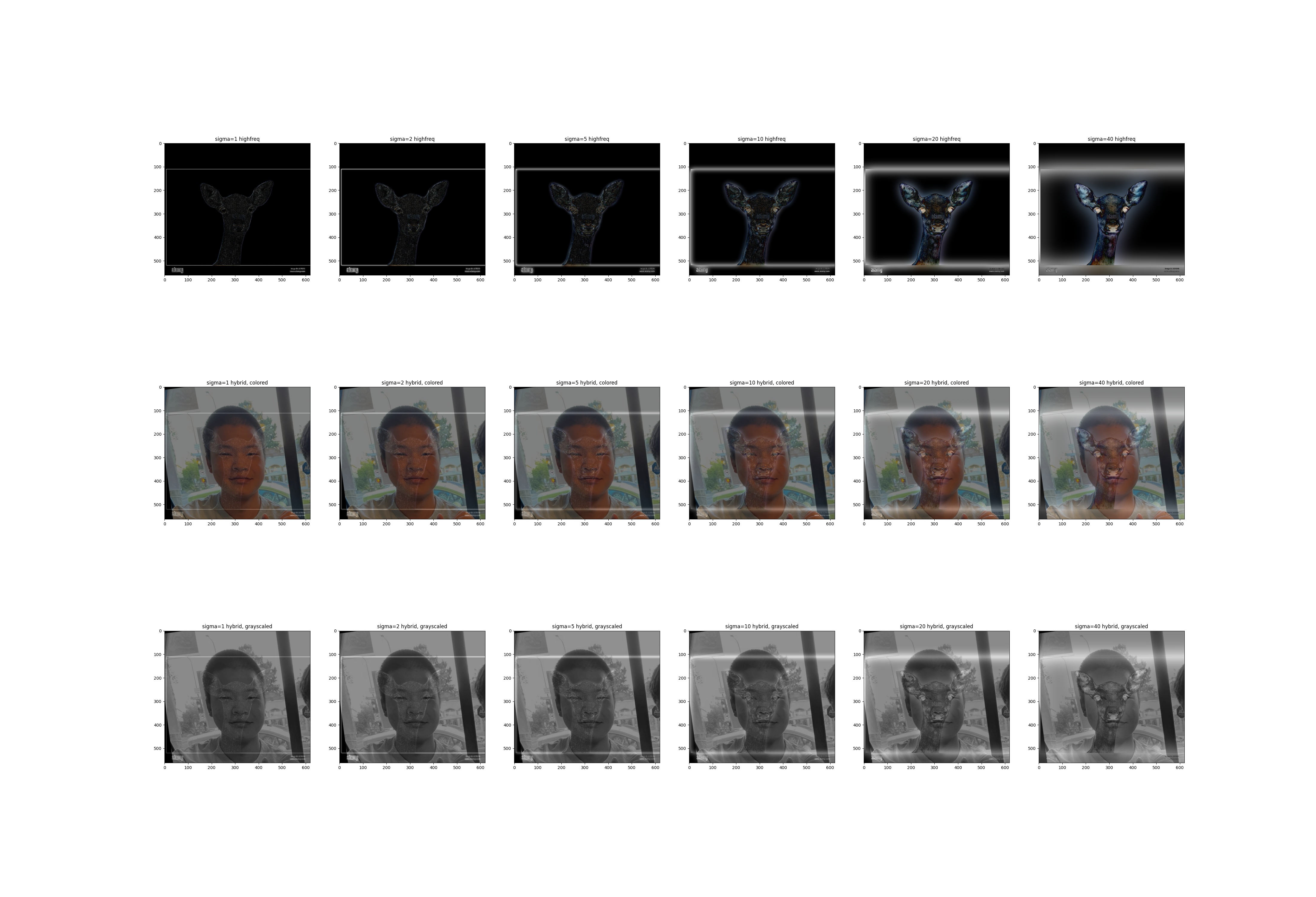

Again, choose a coefficient set of your preference from above to form your favorite deer-ryan. This is inspired by the extensively discussed empirical similarity of Ryan and an anime deer (with some necessary rotations to his face):

Now you may understand why the section is titled this way. The images are not only unbearable to create for its difficult processes, but also unbearable to see, worthy to be called an exercise for both of us writers and readers. Notably, Ryan has posted a picture of my face blended onto the “financial support” meme, and on the other hand, Cyrus hasn’t started the assignment yet.

Fun with Frequencies: Multiresolution Blending

Overview of Methodology

In this task, we concern ourselves with creating absurd entities by blending different images into one, via a Laplacian pyramid that effectively interleaves the details of two pictures with the help of a binary mask. The construction of such pyramids are detailed in the preliminary section at the beginning of this writeup. This submission did not use a stack, we used a pyramid.

In all images, we follow the following procedure to produce our products:

1. Select two pairs of pictures. I already decided that one pair will be about deer and Ryan, so just need to select another pair.
2. Create a mask that can combine the two by background-removal, using image editing tools like Adobe Express/Powerpoint.
3. Hand-refine by a stylus pen.

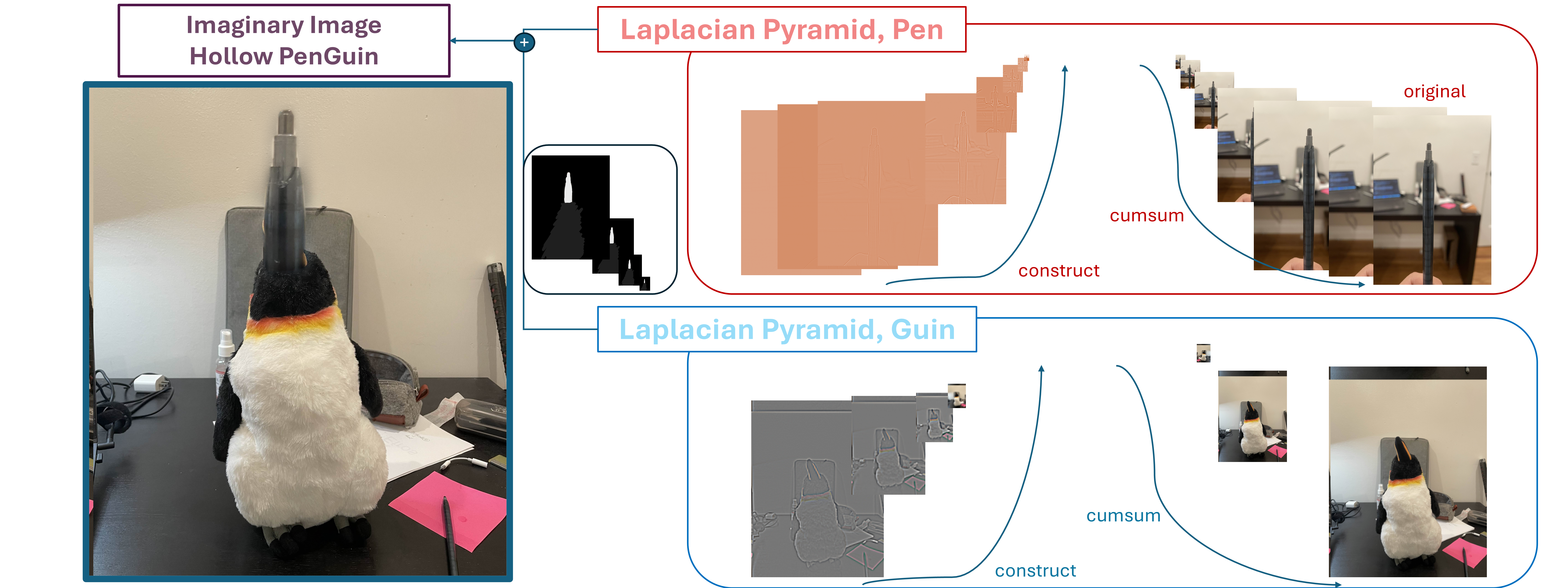
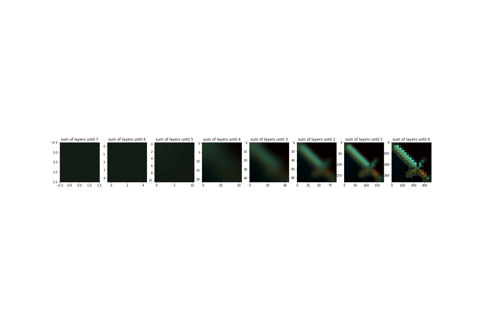
Peeling the Layers of Oraple

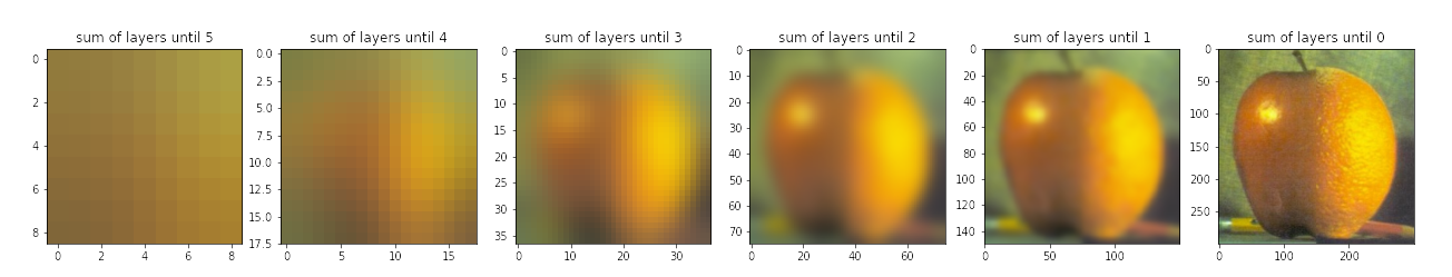
The mask of oraple is simply crafted as a horizontal binary mask. Let us first review the layers of Laplacian pyramids and mask Gaussian pyramid below:

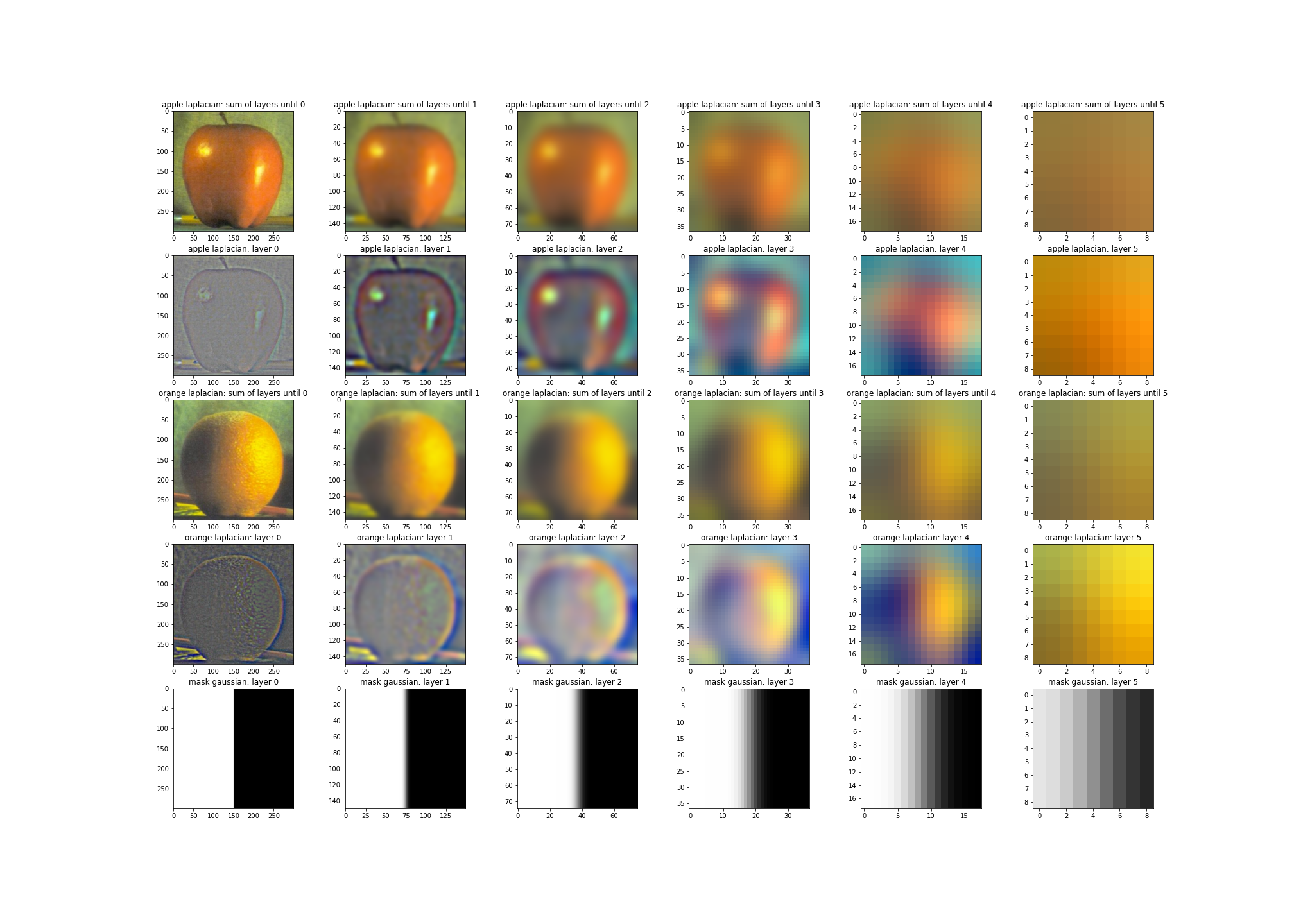
The blended image’s Laplacian layers, without summing, are: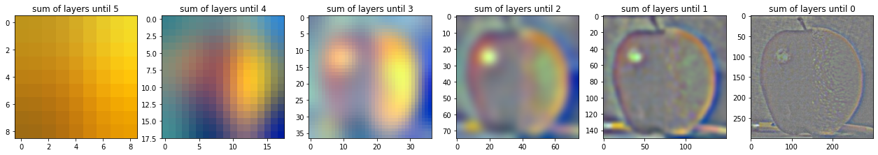

Review the subtitle above each subplot to review what each subplot refers to. Notably, Laplacian layers have been normalized for visibility. Meanwhile, here are some results:

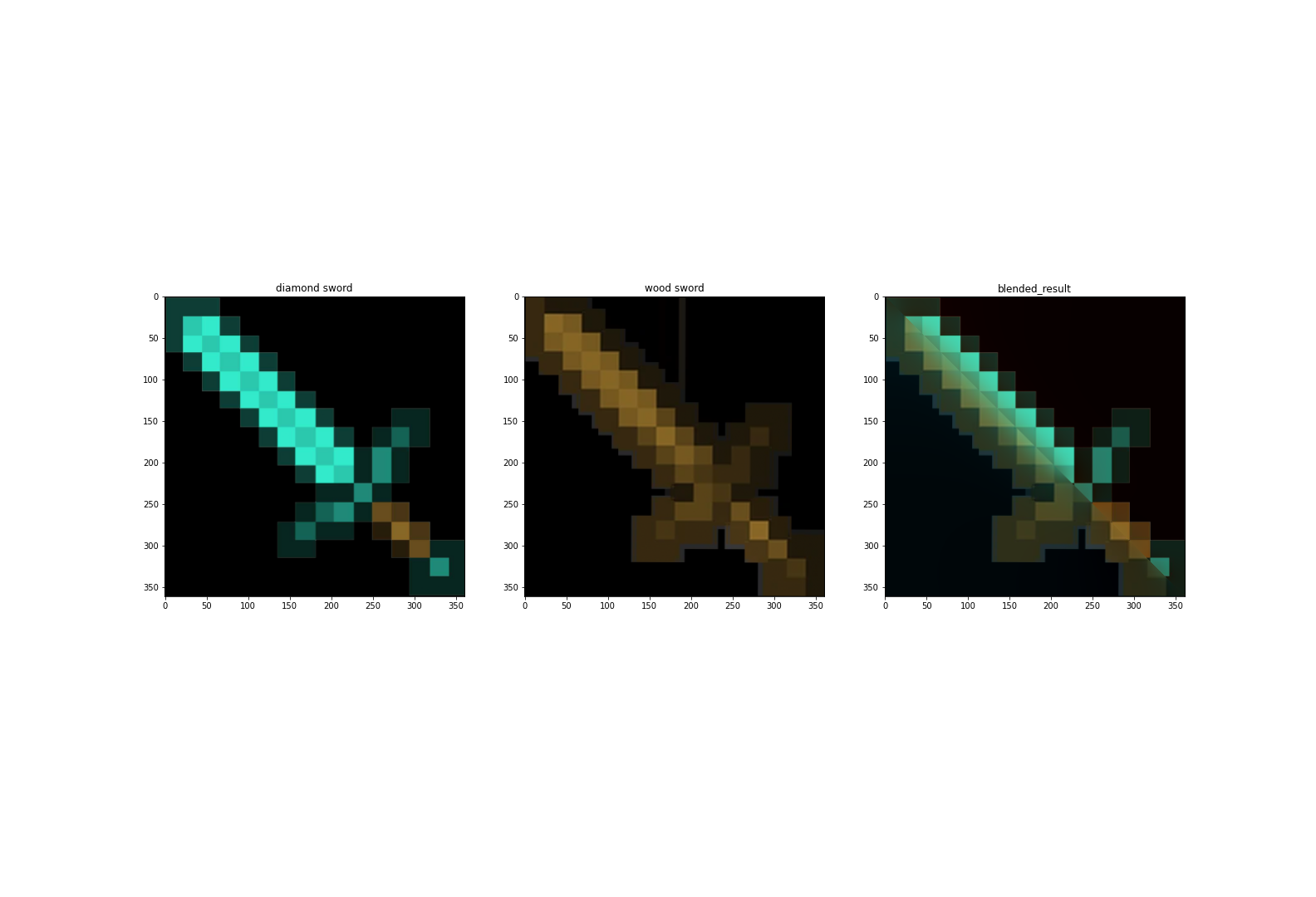
Let us consider another trivial case of blended images with a diagonal binary mask, where I mix two minecraft swords into one.

Irregular Images from Irregular Masks

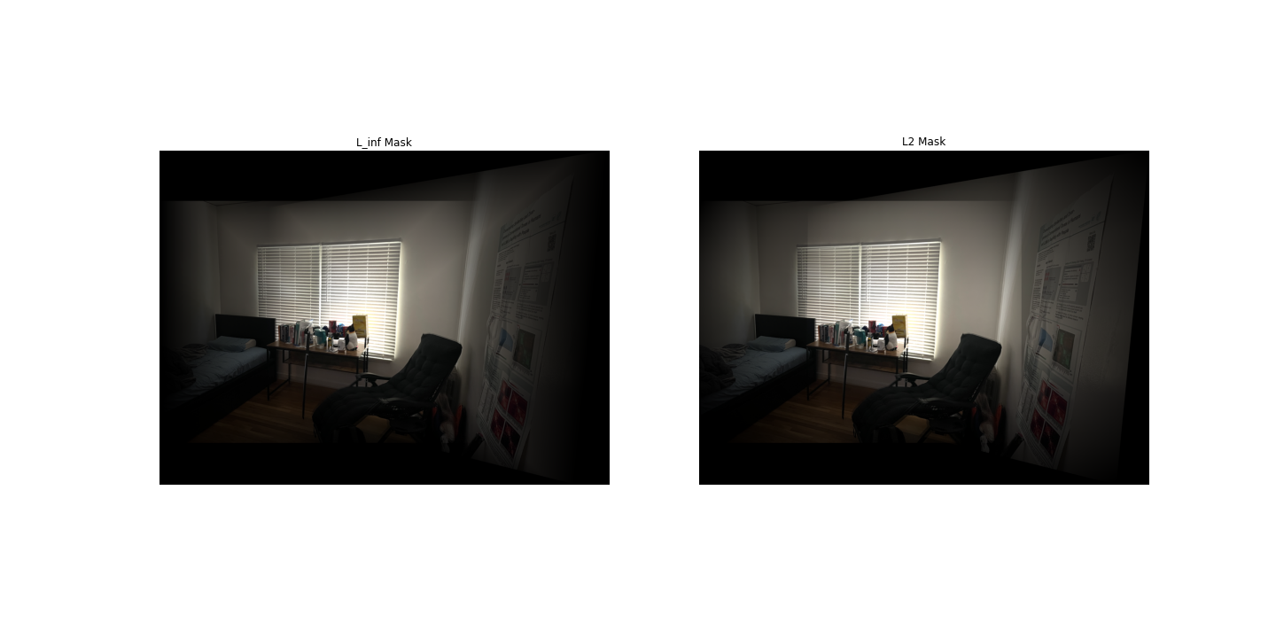
Now, let us consider some cases for irregular masks, where the masks are created based on the apparoach outlined in the first subsection of this section.

Let us first consider a penguin.

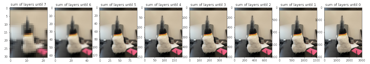
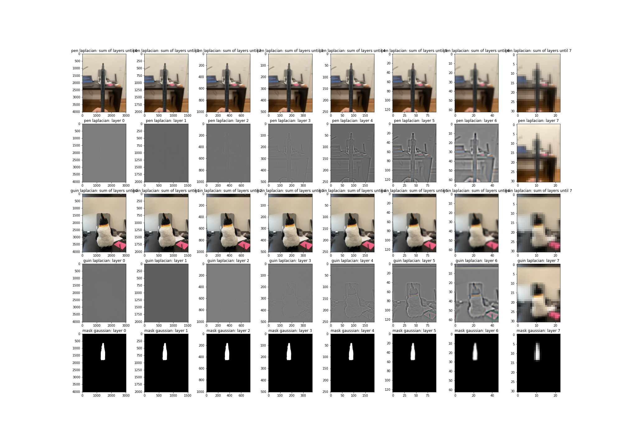
As you see, I blended a pen to a guin.

Now, time for deer Ryan again:

Discussion and Future Work

In this project, I learned the importance of a signal-istic view for images and its application onto image processing. Such view holds great potential for detecting and removing noise for diverse forms of data, potentially applicable for settings that require high data quality, such as deep and reinforcement learning.