COMPSCI 180 Project 4 Writeup

Introduction

In this (rushed) blog post, I detail my doings (and now corrected wrongdoings) in Project 4A (one of them being starting late due to all the other businesses in life).

The assignment discusses image warping and mosaicing. Image warping is a business that we have discussed using a large part of our previous post, while mosaicing is a new topic. What is mosaicing? Mosaicing is stitching two pictures of different perspectives together, forming a panorama of some two sights that have resulted from an observer staying at a fixed global coordinate, but perhaps looking at something from a different angle. An example will be quickly shown in our results section.

We have repeatedly mentioned the word “stitching”, but what really is “stitching”? And how is warpping, an elemental operation for image transformation, related to our works (and my wrongdoings)? We will detail the methodological details of these efforts in the Preliminaries sections, then describe their experimental outcomes using the section following Preliminaries.

Preliminaries of Project 4A

Let us consider a toy example of the two following pictures:

Picture A	Picture B

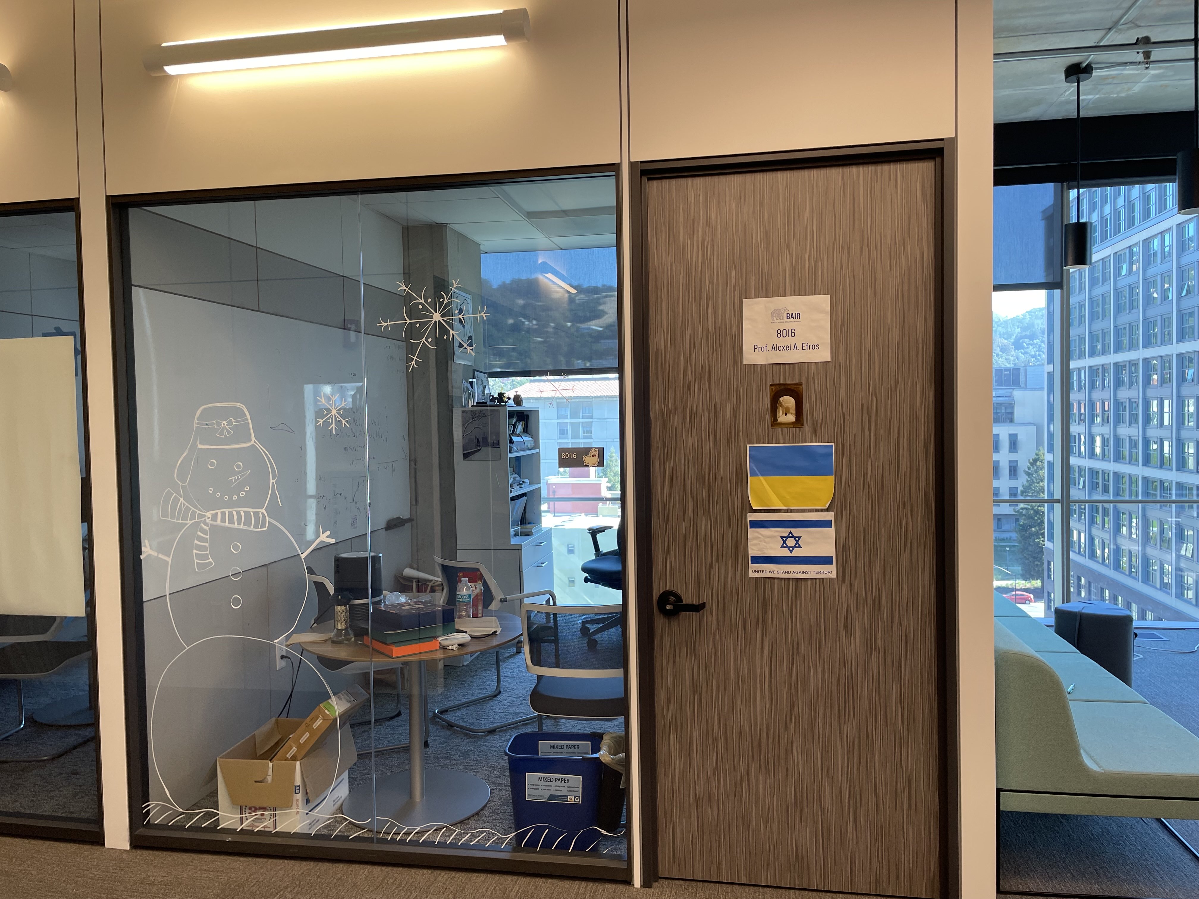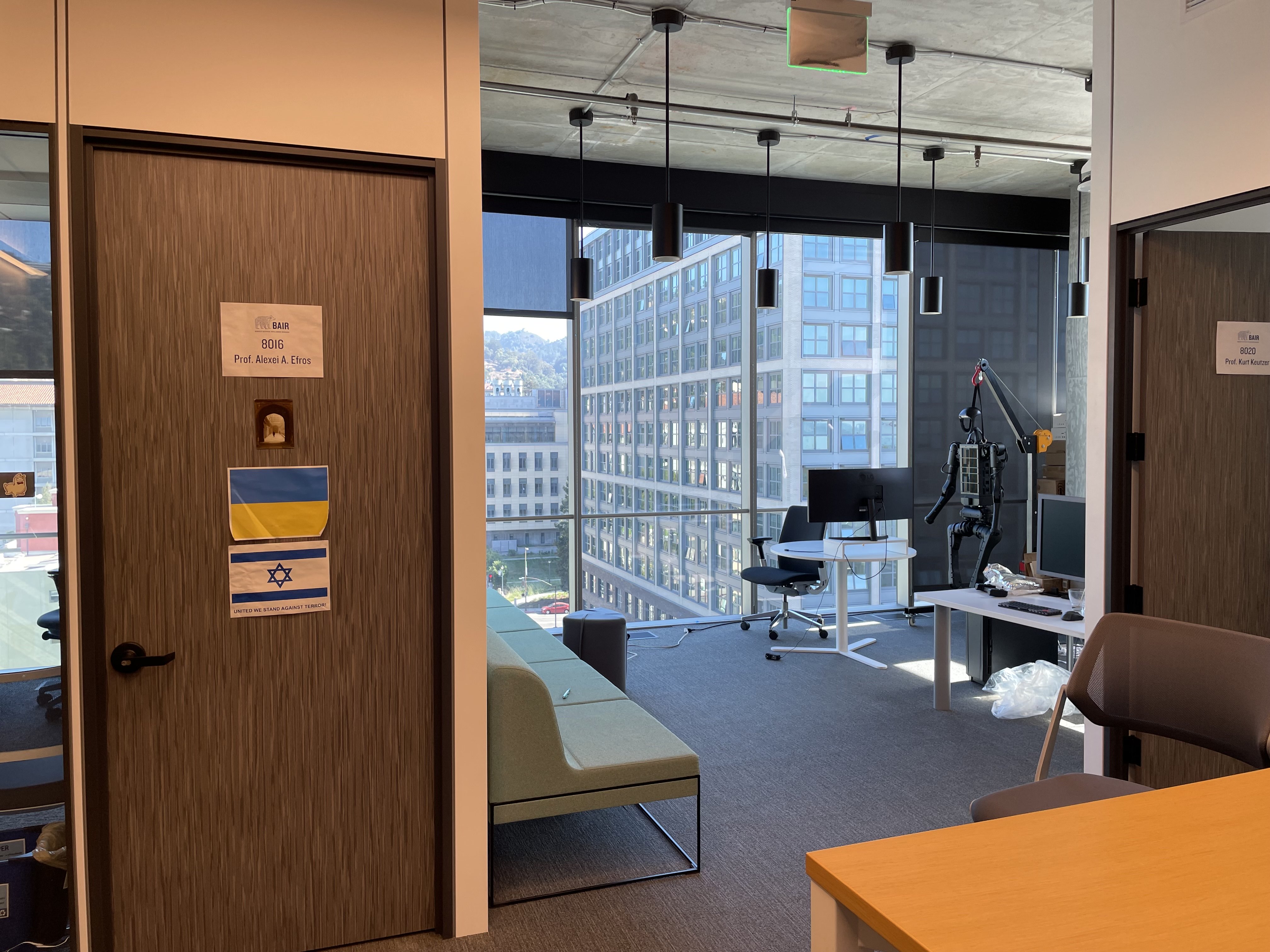These are different views of Prof. Efros’ office seen from the same global coordinate (I stand at the exact same location when looking at these views), but the door’s overall orientation is quite different, because the angle at which I look at the door is different. Therefore, one door is slanted towards the left, and the other is slanted towards the right! Amazing!

So how do we stitch these two pictures together? Well, there is a commonality between these two pictures that we can merge with: the door. Let’s just overlap the images by where the door is… except we can’t just do that. The door’s shapes are different. We must transform, say, Picture B’s door’s shape into that of Picture A’s when we overlap the images (and naturally, all other components follow the same transformation). This is where warpping comes in.

Projective Mapping

In the last blogpost, we discussed finding an affine transformation between two triangles by finding a 3-by-3 transformation matrix via homogeneous coordinates. Here, we concern a different form of transformation: projective transformation.

With at least 4 pairs of $(x, y), (x’, y’)$ as well as the definite assumption that $gx + hy + 1 = w$, we can construct the following system of linear equations and use least squares algorithm to find the optimal estimators for projective mapping parameters:

here, $\mathcal{D}$ is the set of all correspondence points, such as the corners of the door and doorknobs.

Warp2Stitch

Upon obtaining this projection matrix, it’s warping time. The general technique of warpping can be seen at the post for project 3, but I will kindly reiterate it here.

Forward vs. Inverse Warpping

There are two general patterns for warpping: forward-warpping and inverse-warpping.

In forward warpping, once we infer the operator $\mathcal{T}$, we map the value of each pixel at position $(x, y)$ to its transformed equivalent $\mathcal{T}((x, y))$, and non-integer pixel coordinates will have its values distributed among neighboring pixels. However, this pattern of warpping easily leads to “holes” in the resulting product, where certain pixels do not receive any coloration.

Therefore, our assignment proceeds with an alternative method: inverse warpping. In this paradigm, we infer an operator $\mathcal{T}$ from the source image to a target image, and use the inverse operator: $\mathcal{T}^{-1}$ to do pixel mapping as described above. However, since the source image’s pixel values are all known, we can safely interpolate the unknown pixel values with its neighbors. An efficient manner of doing so is bi-linear interpolation, where for each $(x_t, y_t) = \mathcal{T}^{-1}(x, y)$ resulted, its coloring is inferred as a weighted sum of its neighbor. In our assignment, we apply a variation of this logic that will be described below (out of the unclarity of the original assignment’s instruction, we devise a variation of this interpolation function fitting our context).

Constructing the Blending mask

To construct a smooth transitioning blending mask, we will formulate our mask with the following procedure:

1. Predefine masks whose pixel values are equivalent to the distance between themselves and the nearest edge, then normalize the mask.
2. Warp them with their corresponding images.
3. Construct the final mask as an aggregation of mask for image A and B such that each pixel of the mask has intensity $\frac{\alpha_a}{\alpha_a + \alpha_b}$ for the final mask of Image A, and similarly for Image B with $\frac{\alpha_b}{\alpha_a + \alpha_b}$.
4. Multiply each warpped image by their corresponding final mask, then add the masked images together. Thanks Ryan!

Overall Flow of Methodology for Warping

The overall flow of mosaic would then seem as follows:

1. Obtain the homography transformation via least squares to match correspondences from Picture B to Picture A
2. Transform the corners of Picture A onto Picture B, seeing where it will generally land.
3. Take a polygon mask using the transformed corners, and obtain all integer coordinates for pixels in there.
4. Inverse warp onto the transformed polygon mask mentioned in (3), and use bilinear interpolation to fill in the mask
5. Use an infinity-norm based distance transform mask to blend the two images. A Laplacian kernel would be much preferred, but I need to go revise exam logistics and write SoPs.

Preliminaries of Project 4B

Feature Detection

To detect features that are helpful for alignment, we can consider first what kind of features are best as correspondence points between two images. And that is corners. Corners of a door, or a wall, can often represent a distinct boundary between some objects, and is therefore distinctive of the geographical location of something in a picture. Therefore, when automatically detecting features, we don’t want to cut corners, but we want to find corners.

The Harris corner detector described in lecture (which you should go to) fulfills this purpose with the simplified procedure below:

1. Calculate the gradient of the image as $I_x$, $I_y$.
2. Construct the structure tensor matrix, known as $M = \begin{bmatrix} I_x^2 & I_x I_y \ I_x I_y & I_y^2 \end{bmatrix}$, which provides us a structural summary of the change at pixel.
3. With reasons not mentioned here, we learn that the eigenvalues of $M$ provide us knowledge of what’s a corner. A corner occurs at a pixel whose matrix has two large eigenvalues, such that $R = \det (M) - k ({\rm trace}(M))^2 > 0$.

Now, then, we get a set of pixels that can be Harris corners based on peak-finding algorithms.

However, is a pixel a good feature because it is a Harris corner, or is the pixel a Harris corner because it is a good feature?

The answer is, a pixel is a Harris corner because it’s a potentially good feature, but it might not be useful, because it can be a not-so-prominent peak within the space of $R$ values throughout pixels. Therefore, we use an additional technique called Adaptive Non-Maximal Suppresion (ANMS) to filter the Harris corners down to a set of $250$ or $500$ points.

The ANMS algorithm follows as:

1. For each Harris corner, compute its minimal suppresion radius as $r_i = \min_j d(x_i - x_j)$ where $f(x_i) < c_{robust} f(x_j)$ for an $x_j$ being one of the Harris corners.
2. Pick the $n$ pixels with the largest values for $r_i$.

Therefore, upon applying ANMS, we know throughout the Harris corners and the suppressed points, these 500 pixels alone are the promising features.

Feature Matching

Patch Descriptor

To describe a feature (a pixel, a corner), we can use an 8x8 patch around it by sampling with stride 5. That is, for a pixel at $(x, y)$, the pixels we sample as its descriptors can be described with the set of points

Well, this forms a 9x9 patch, but would I re-formulate a piece of working code to make it work again under this subtle imprecision that doesn’t affect my final result? Nah, I’d continue writing the blog post. The patch also needs to be standardized.

Nearest Neighbor Matching

To match features across image A and B, we can first find nearest neighbor matches of them. That is, we first construct a nearest neighbor instance for features in image A and B, then we see what pairs of features across images A and B are each other’s nearest neighbor. Then, among those points, we filter out all pairs whose following statistic is less than $0.5$ (the paper suggests $0.4$, but I made it more generous judging by my data):

Surprisingly, my implementation doesn’t use a Nearest Neighbor data structure from any existing libraries. I just use a cdist distance matrix between feature patches.

RANSAC

Lastly, the RANSAC algorithm can be described as an iterative process as follows, which helps us find the largest set of inliers that constructs the homography we want for our eventual warping and stitching procedure.

1. Take a deep breath for the upcoming code you have to write.
2. initialize best_error, best_inlier_set.
3. Iterate the following procedure for $n=1000$ times:
   1. Select four random pairs without replacement
   2. Compute the homography $H_i$ for these four random pairs.
   3. Record the set of pairs such that when applied this homography, the distance between the transformed feature of image A and the corresponding feature of image B are less than 2 pixels away.
   4. If the error of homography is smaller than best_error and we have encountered the biggest inliner_set up to now, record our homography and inliner_set, and update our best_error.

Then, you may stitch proud, as your features are aligned.

Rectify and Justify

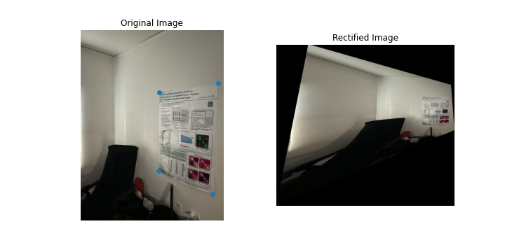
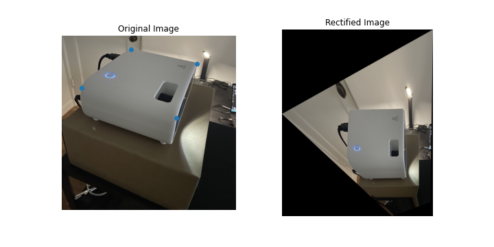
To make sure our warpping implementation is intact, we would like to try rectifying some aspects of an image, such that a specific set of four pairs of correspondence points should form a square or rectangle in a warpped image.

The results are as follows:

Sike, it’s Mosaic

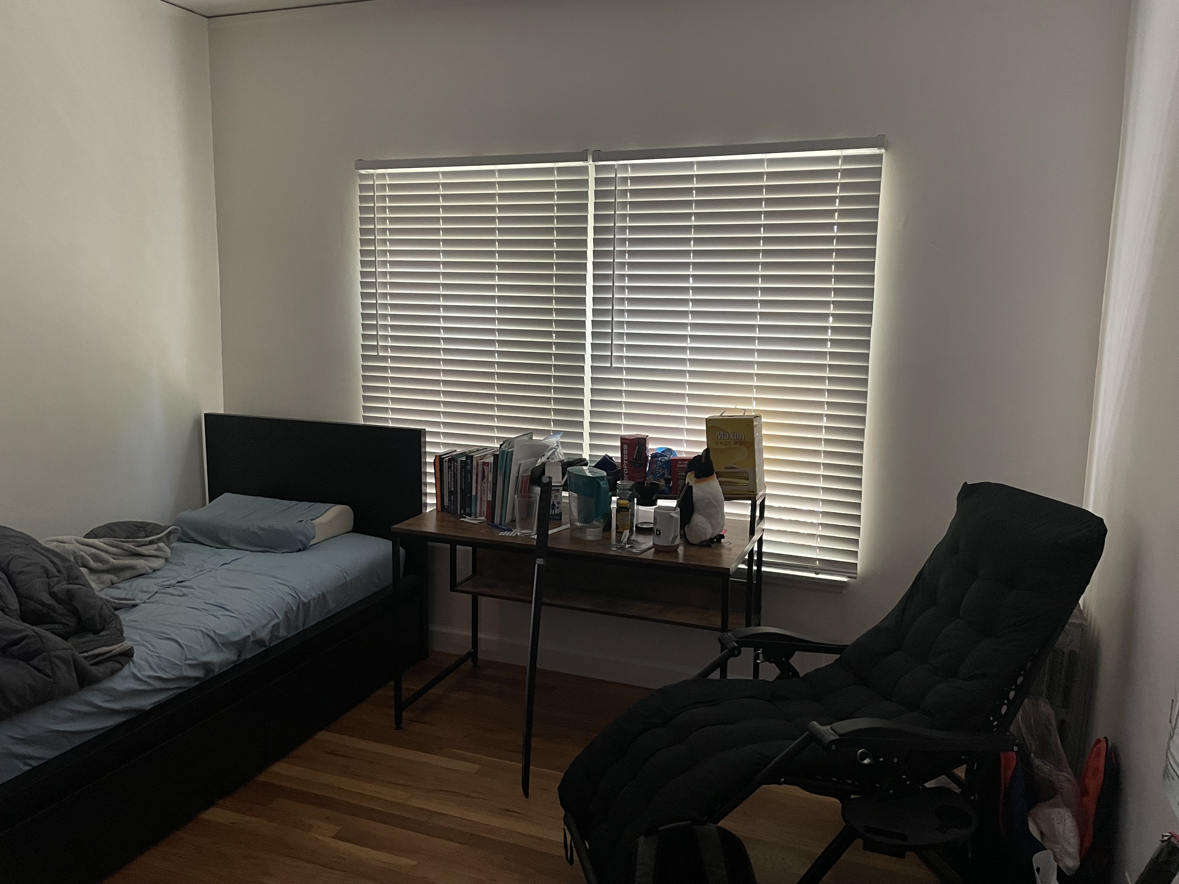
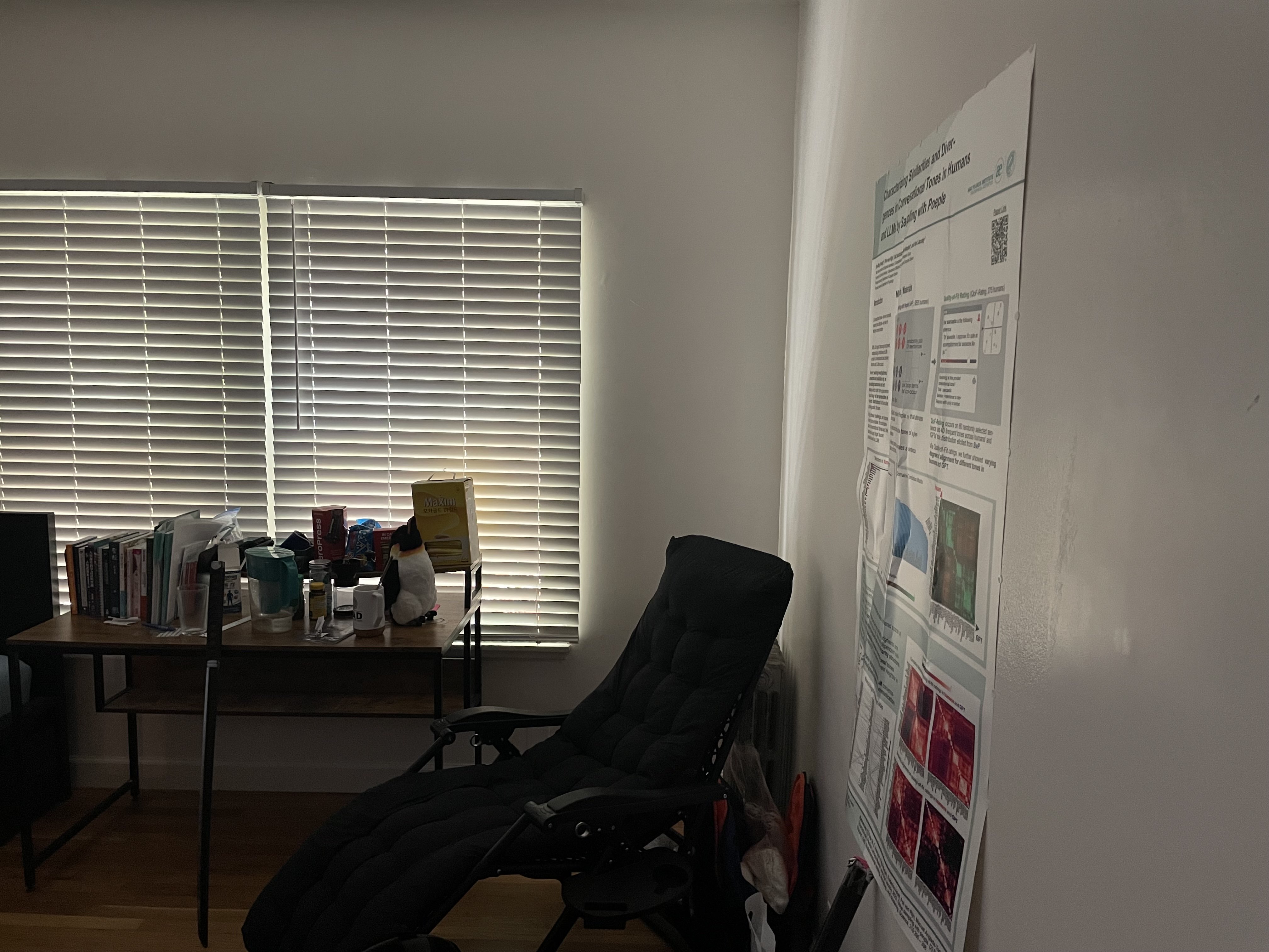
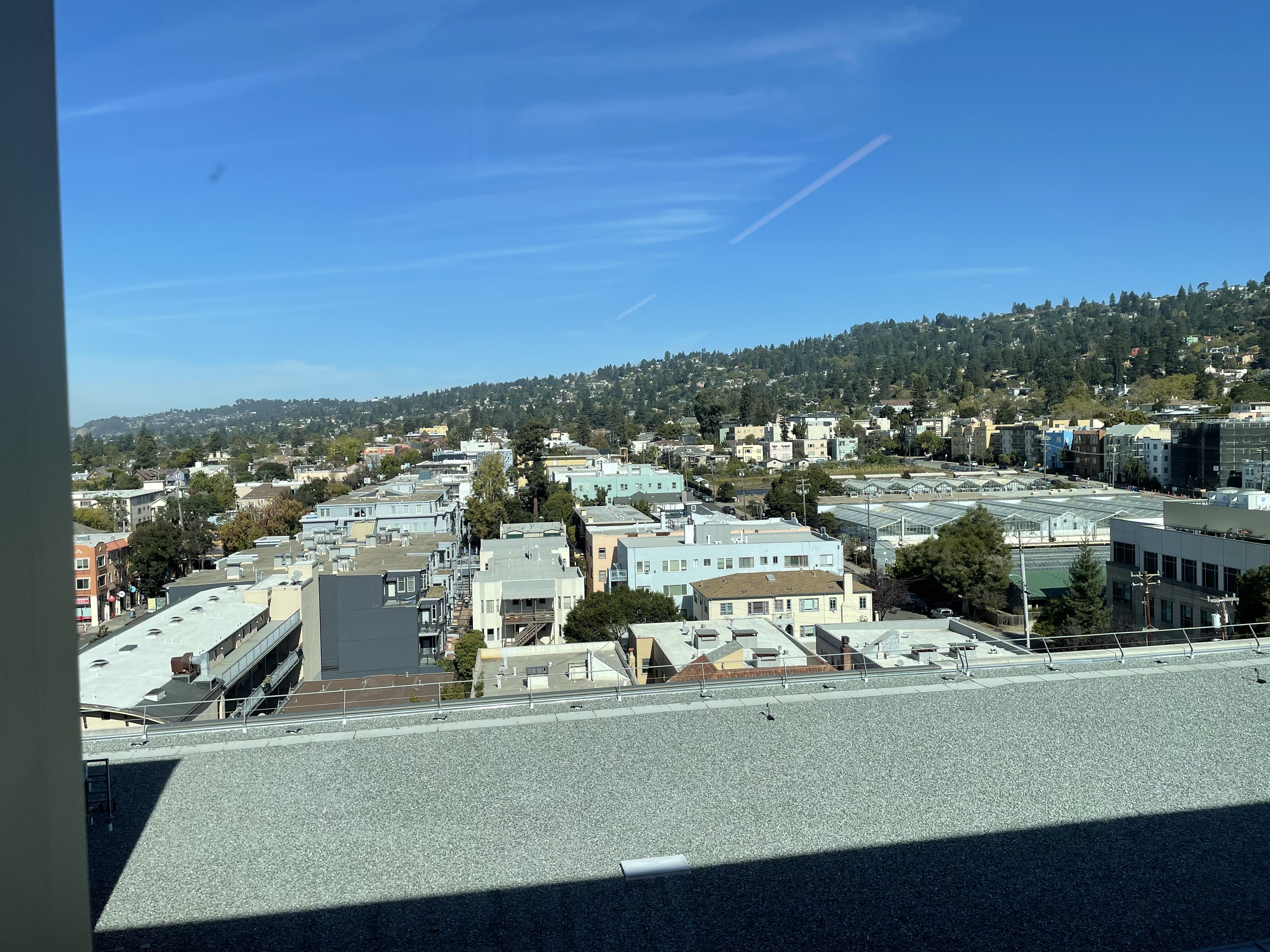
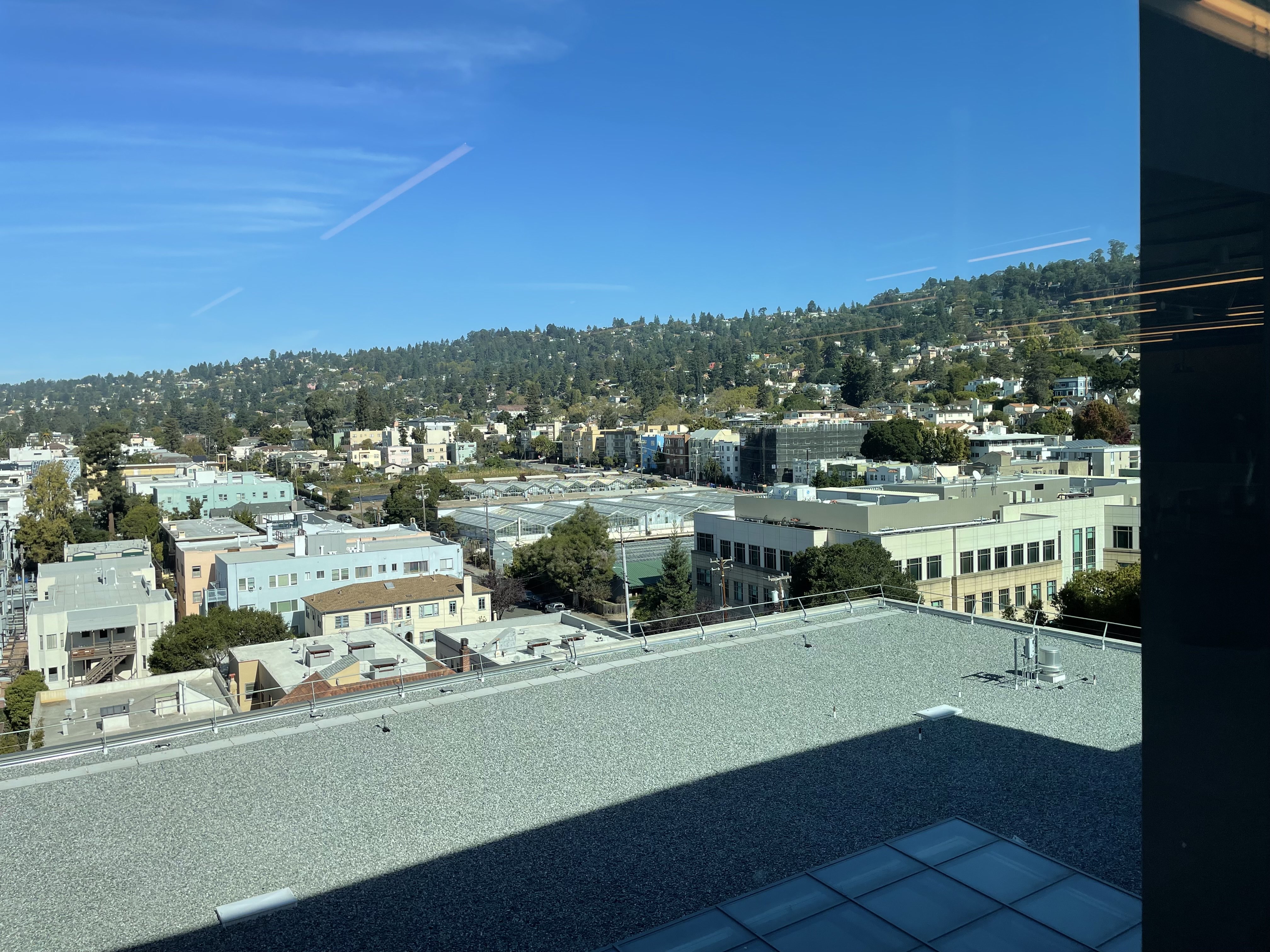
Here are the mosaics.

Original Picture A	Original Picture B

Results:

Original Picture A	Original Picture B

Results: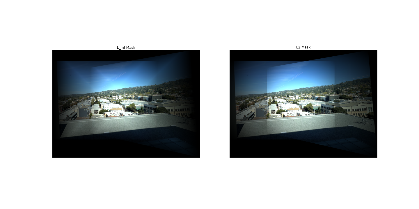

Original Picture A	Original Picture B

Results: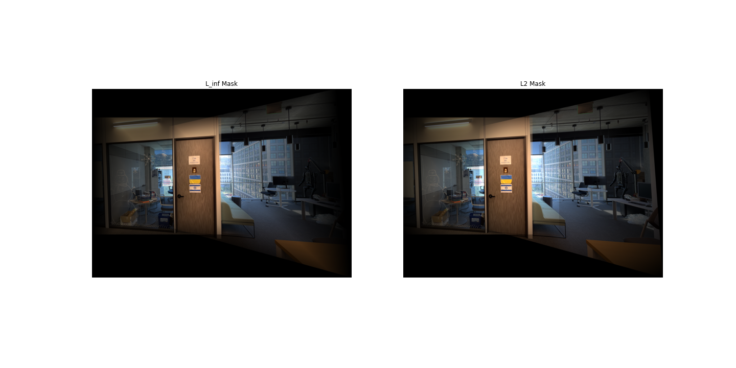

Generally, the results match in structure. The color differences may be efficiently resolved using a Laplacian kernel, or be more careful when taking pictures.

Automatic Feature Discovery

Feature Detection: Harris Corners and ANMS

The Harris corner filled my entire picture for any instances, so I’ll showcase my ANMS points here instead!

As you can see, they be zoomin. Therefore, we should suppress more of them with the matching procedure.

Feature Descriptor, Matching, RANSAC

Example patches of feature detectors for picture C1 is shown below:

As you can see, the corners on the flag posted on Prof. Efros’ door has brought some attention to our feature detector!

Furthermore, here are the true inliers found by RANSAC on each image after their nearest neighbor matching procedure discussed in the Preliminaries for 4B section above.

The Outcome of Three Slip Days

ITS STITCHING TIME!

What have I learned?

It’s cool to automatically find features (even though the methods are complicated), and now I appreciate representation learning a bit more for finding these by itself.