[COMPSCI 180] Project 5: I Forward, I Denoise, I Diffuse
Published:
COMPSCI 180 Project 5 Writeup
Project 5A: The Applications of Diffusing
The random seed used at here is always 180.
Setup Procedures
To set up for this project, we need to:
- Acquire access to a text-conditioned diffusion model. This assignment uses the DeepFloyd IF diffusion model.
- Organize the upsampling code in the notebook.
- Precompute the text embedding of several image prompts to be used later.
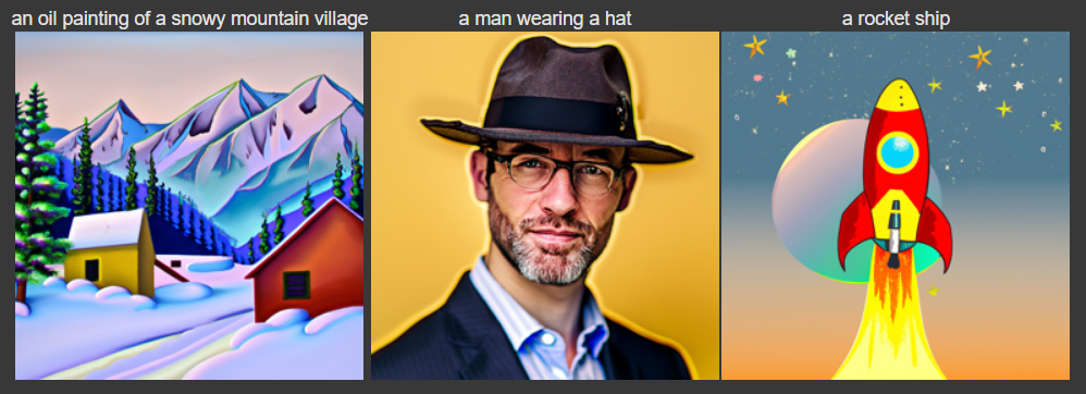
Here is a demonstration of the prepared model’s capabilities with inference step $20$:
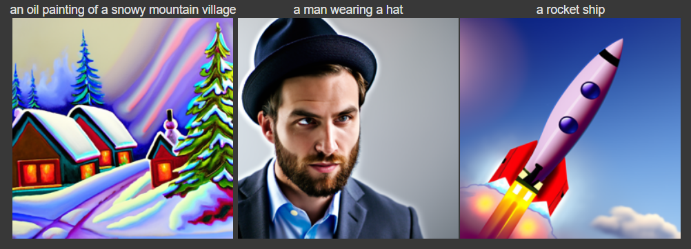
and with inference step $40$:
Preliminaries
Diffusion models are generative models that create samples from a distribution via learning to denoise some noised version of an image.
Particularly, we would denote $x_0$ as an object that is completely clean, such as a picture that we want to generate. Then, the intuition of learning a diffusion process is that we would observe how adding noise destructs the appearance of an image. This is known as a noising process, where we proceed from $x_t$ to $x_{t’ > t}$.
By observing the reversed trajectory of that destruction process, we learn the generation process, going from $x_{t’ > t}$ to $x_t$. The name of this process comes from its literal interpretation– it’s a denoising process.
Specific equations formulate these processes, normally with the help of normal random bariables $\mathcal{N}$.
Implementing the Forward Process [1.1]
The forward process, also known as the noising process, is defined as:
\[q(x_t | x_0) = \mathcal{N}(x_t; \sqrt{\bar{\alpha}} x_0, (1 - \bar{\alpha_t}) \mathbf{I})\]Be very cautious that $\mathbf{I}$ is a matrix of $1$s, not an identity matrix. This comes from the primitive form of generating $x_t$:
\[x_t = \sqrt{\bar{\alpha}} x_0 + (1 - \bar{\alpha_t}) \epsilon, \epsilon \sim \mathcal{N}(0, 1)\]Throughout the post, we will be using this test image quite often, so remember its existence…

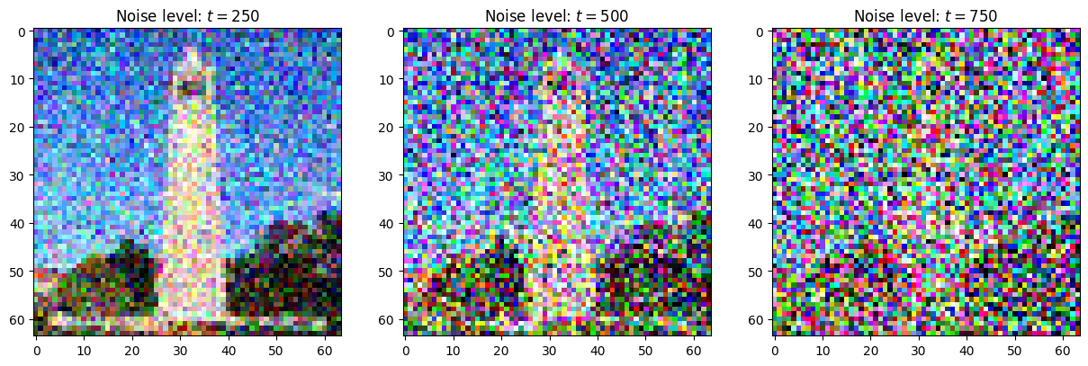
Implementing this procedure with $t \in [0, 999]$ on images with height and width of $64$, we obtain the following results as we noise the image for a different amount of timesteps:
Classical and One-Step Denoising [1.2, 1.3]
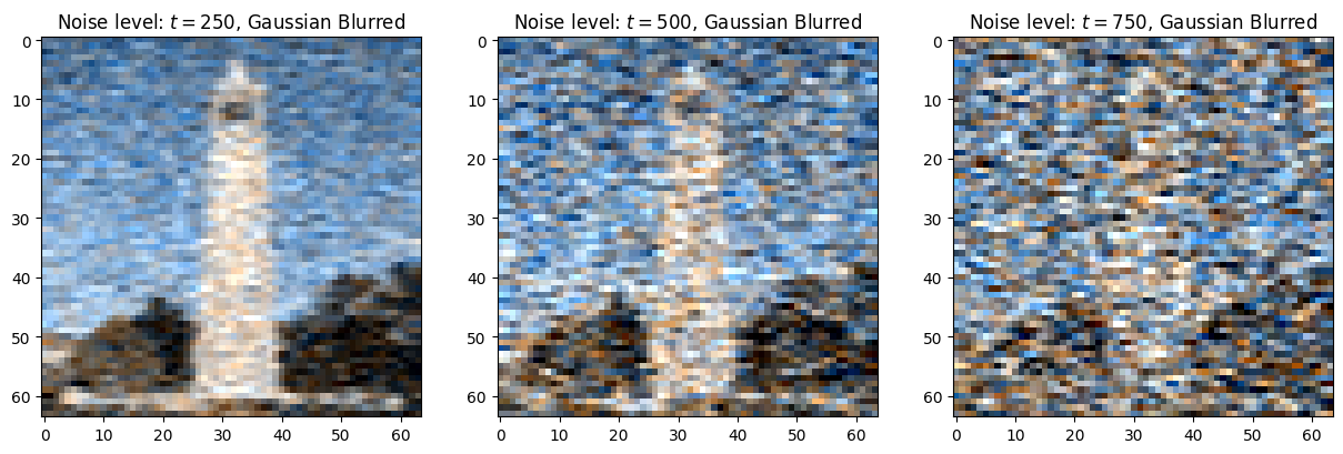
By applying a Gaussian blur, we hope to remove the noise in an image. However, its results are unideal when the image is very nosiy:
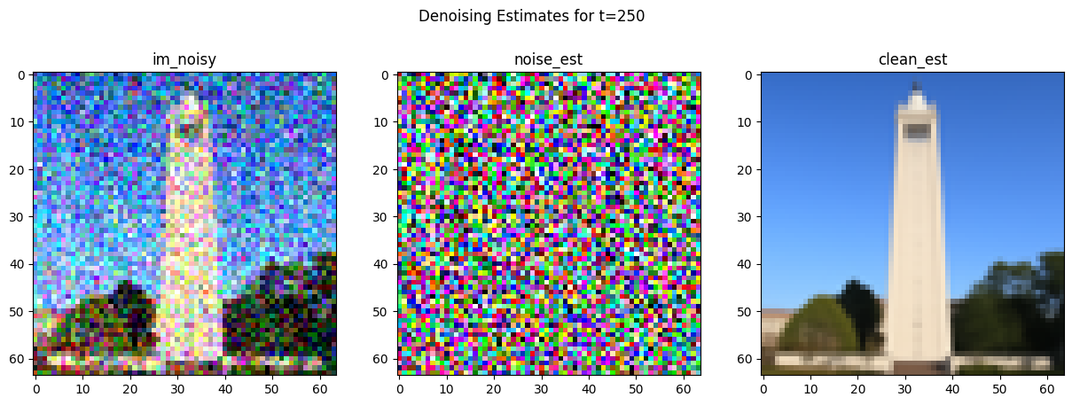
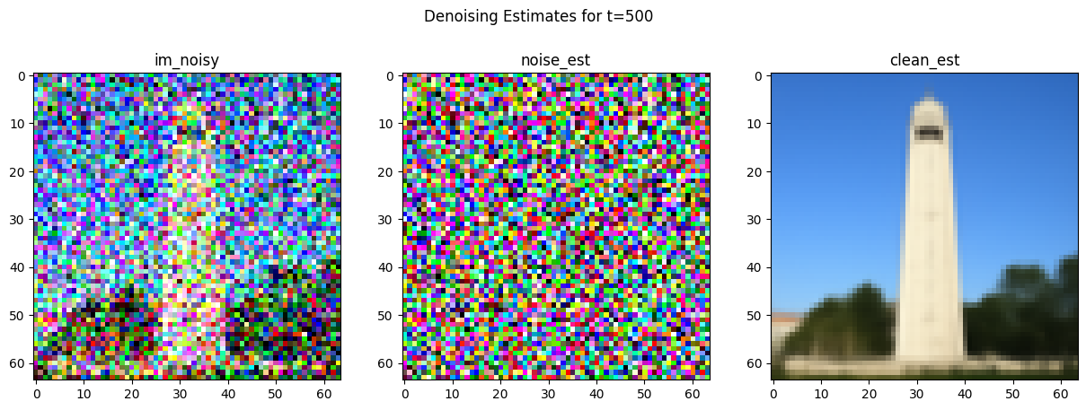
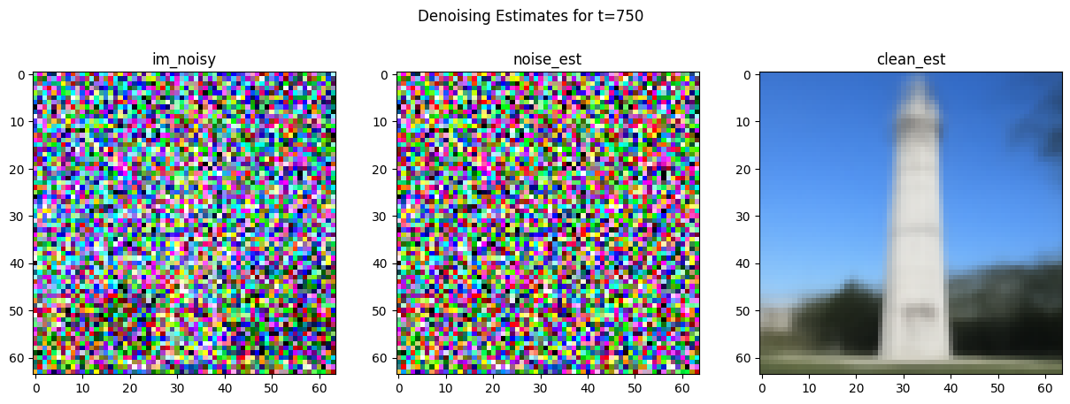
But if we instead try to estimate the noise using the UNet of our diffusion model, then we can achieve an effective estimation of the clean image:
Iterative Denoising [1.4]
Having to denoise through $1000$ steps is costly. Recent work has discussed the possibility of one-shot diffusion, but I haven’t read the paper, so here’s an okay cheap alternative to that. We can use strided timesteps, which can scale the amount of timesteps required down by roughly threefold. Particularly, the noisy image at timestep $t$ now becomes:
\[x_{t'} = \frac{\sqrt{\bar{\alpha}_{t'}} \beta_t}{1 - \bar{\alpha}_t} x_0 + \frac{\sqrt(\alpha_t) (1 - \bar{\alpha}_{t'})}{1 - \bar{\alpha}_t} x_t + v_{\sigma}\]the definitions of these variables can be found in the instructions. This strided timestep works as an interpolation trick.
Here is a view of the noising process:

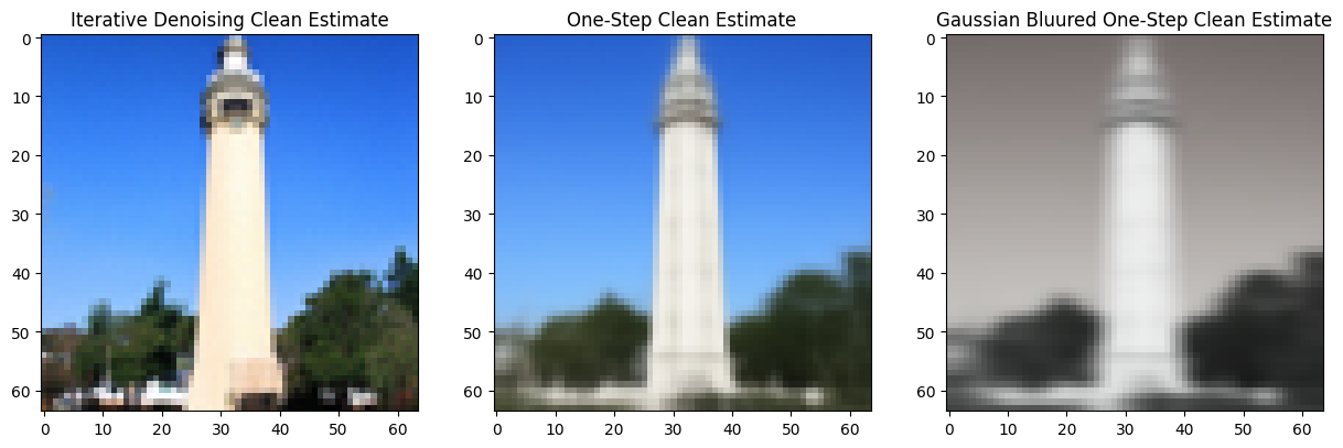
And here is a comparison of the denoised results via diffusion and classical approaches:
Diffusion is Your Friend with Conditions [1.5, 1.6]
To sample from the distribution of images that our diffusion model models, we can step through the entire denoising trajectory by starting with images composed of purely random noise.

Interestingly, involving a classifier-free guidance by using noise estimates from conditioned and unconditioned prompts can improve our image quality. Let $\epsilon_c$ be the conditioned noise estimate (where there is an existing prompt we’d like), and $\epsilon_u$ be the unconditioned noise estimate (in our context, it is the noise estimate for a null empty prompt). Then, the new estimate is experssed as:
\[\epsilon = (1 - \gamma) \epsilon_u + \gamma \epsilon_c\]where the hyperparameter $\gamma$ is free of choice and encouraged by the assignment to be $7$. The samples of this method observe a much higher quality:

Image-to-Image Translation [1.7]
From this point forward, we will benefit all of our approaches with the use of CFG. The first application we’d like to try out is image-to-image translation, which demonstrates a process of arbitrary images slowly leaning towards looking alike to an originally provided image:
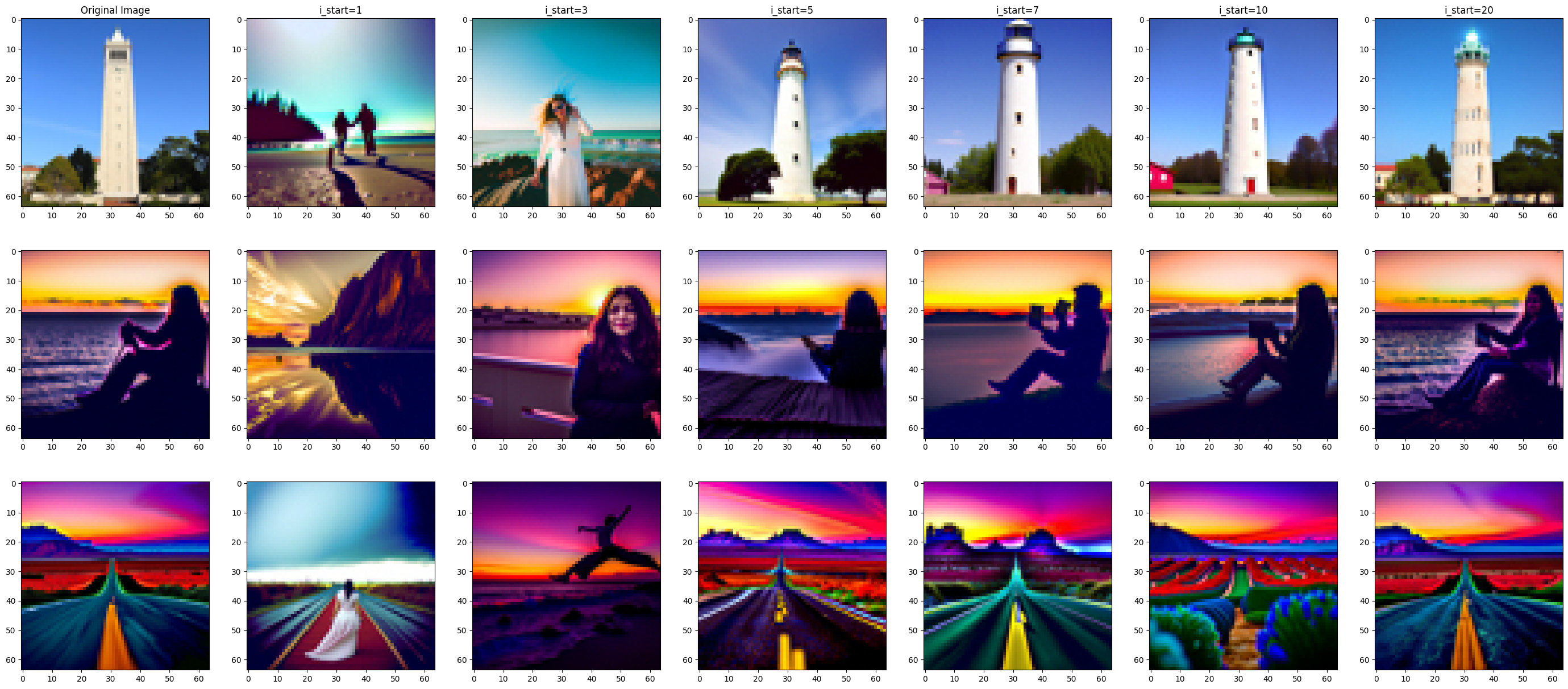
This procedure is otherwise known as SDEdit.
We can also apply this trick on web images and hand-drawn images to make it high-quality photos in intermediate steps.
Web image:

SDEdit Results:

Hand drawn image A:

SDEdit Results:

Hand drawn image B:

SDEdit Results:

Impainting [1.7]
Impainting is a trick where we only provide diffusion for an unmasked region of the image, allowing for a portion of the image to be altered. To put this into mathematical formulation, at obtaining $x_t$ for each $t$, we apply the following update as well for a mask $\mathbf{m}$ that is $1$ where new contents should occur:
\[x_t \leftarrow \mathbf{m} x_t + (1 - \mathbf{m})~{\rm forward}(x_{orig}, t)\]Here are some possible results of this technique:
Setup A: 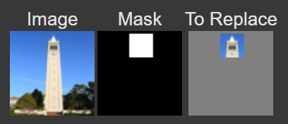
Result A: 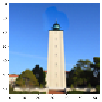
Setup B: 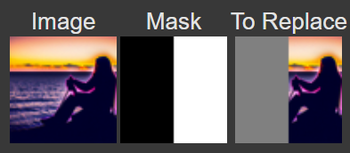
Result B: 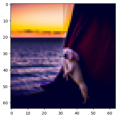
Setup C: 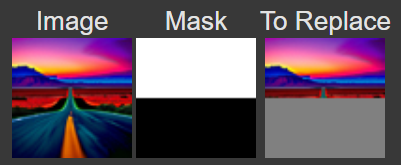
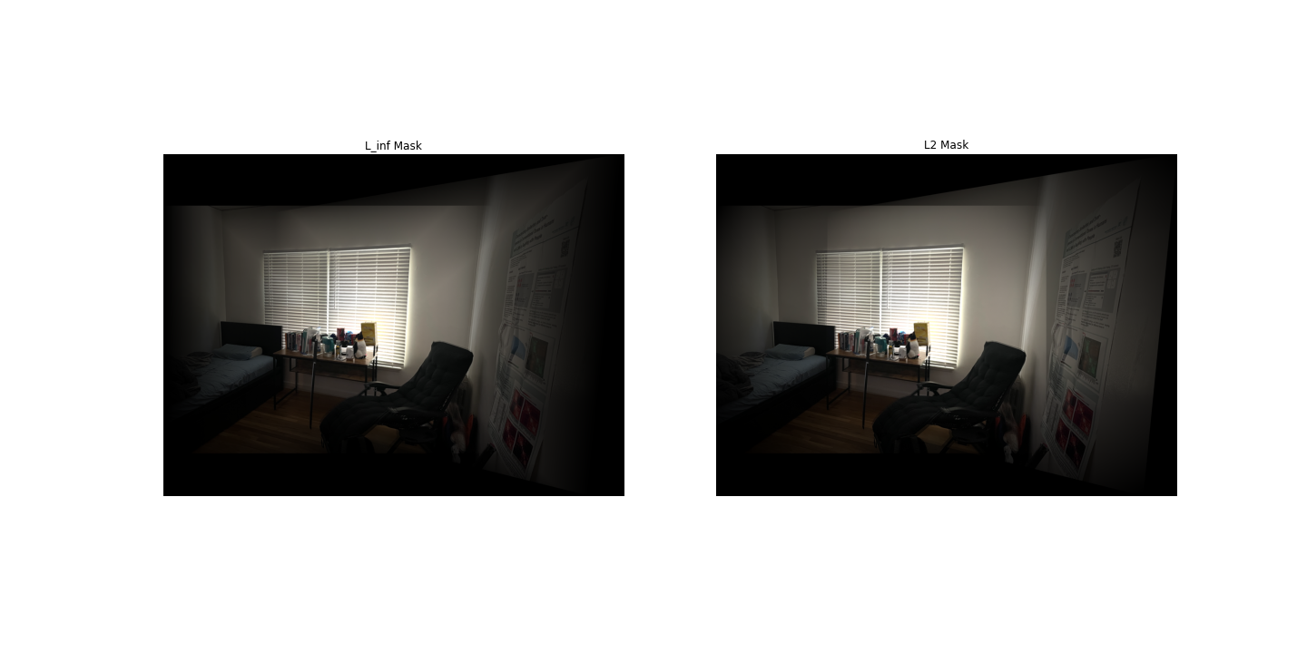
Result C: 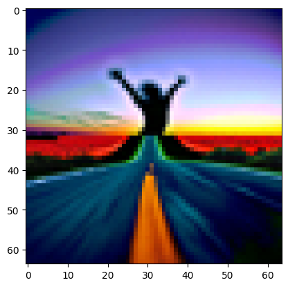
Text-Conditional Image-to-Image Translation [1.7]
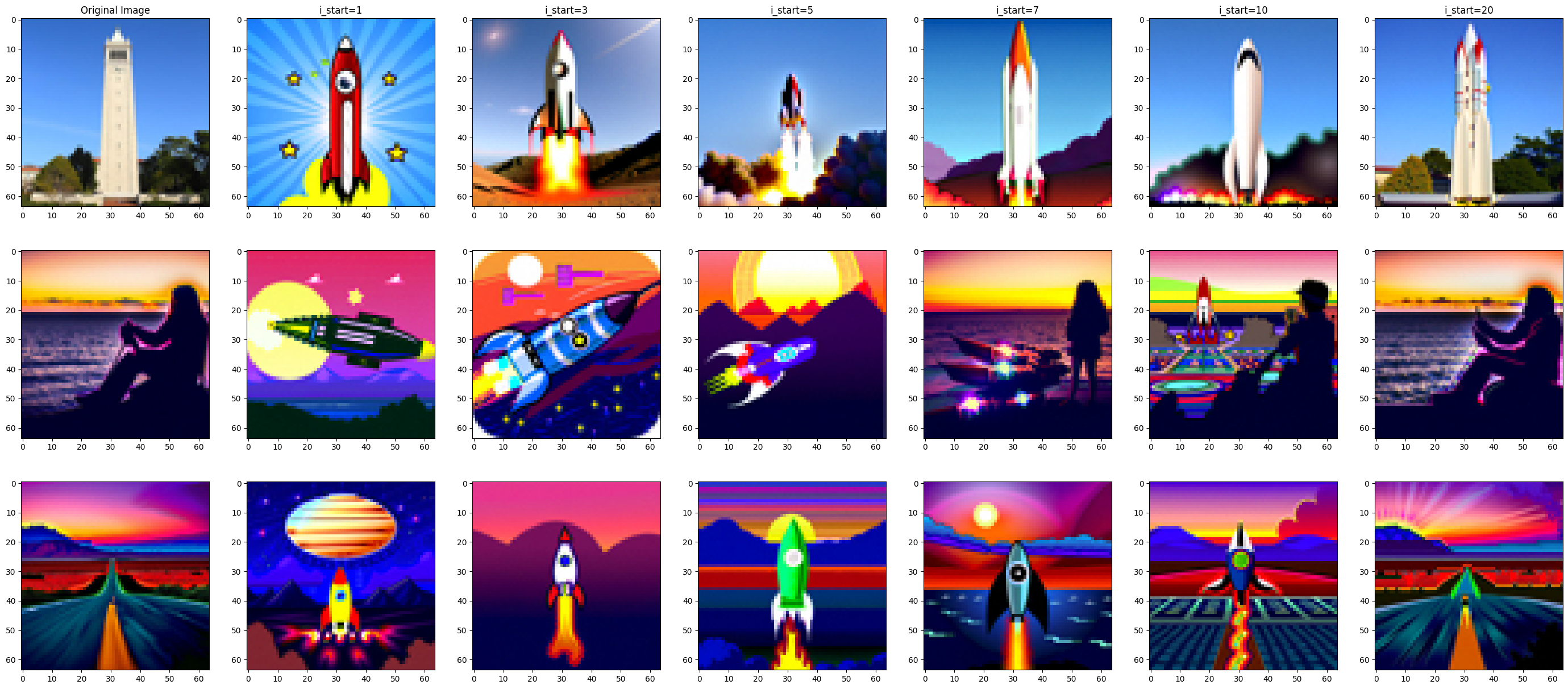
We can also let images shift from one prompt’s content to another by changing the conditioned prompt from “a high quality photo” to something else, like “a rocketship”. Here are some example outputs of the technique:
Visual Anagrams [1.8]
Visual anagrams can be produced by mixing class-conditioned noises of each text prompt. The full algorithms is noted at the assignment instruction, although it misses the CFG part of the formulation.
Here are some results:
Prompt: “an oil painting of an old man” flips into “an oil painting of people around a campfire”

Vertically flipped:

Prompt: “a lithograph of waterfalls” flips into “a lithograph of a skull”

Vertically flipped:

Prompt: “an oil painting of a snowy mountain village” flips into “a photo of a dog”

Vertically flipped:

Hybrid Images [1.9]
Back to making hybrid images! To do so, similarly follow the instructions, but instead of having separate unconditioned noise estimate, use one unconditioned noise estimate with the sum of noised estimates to perform CFG-styled noise estimation.
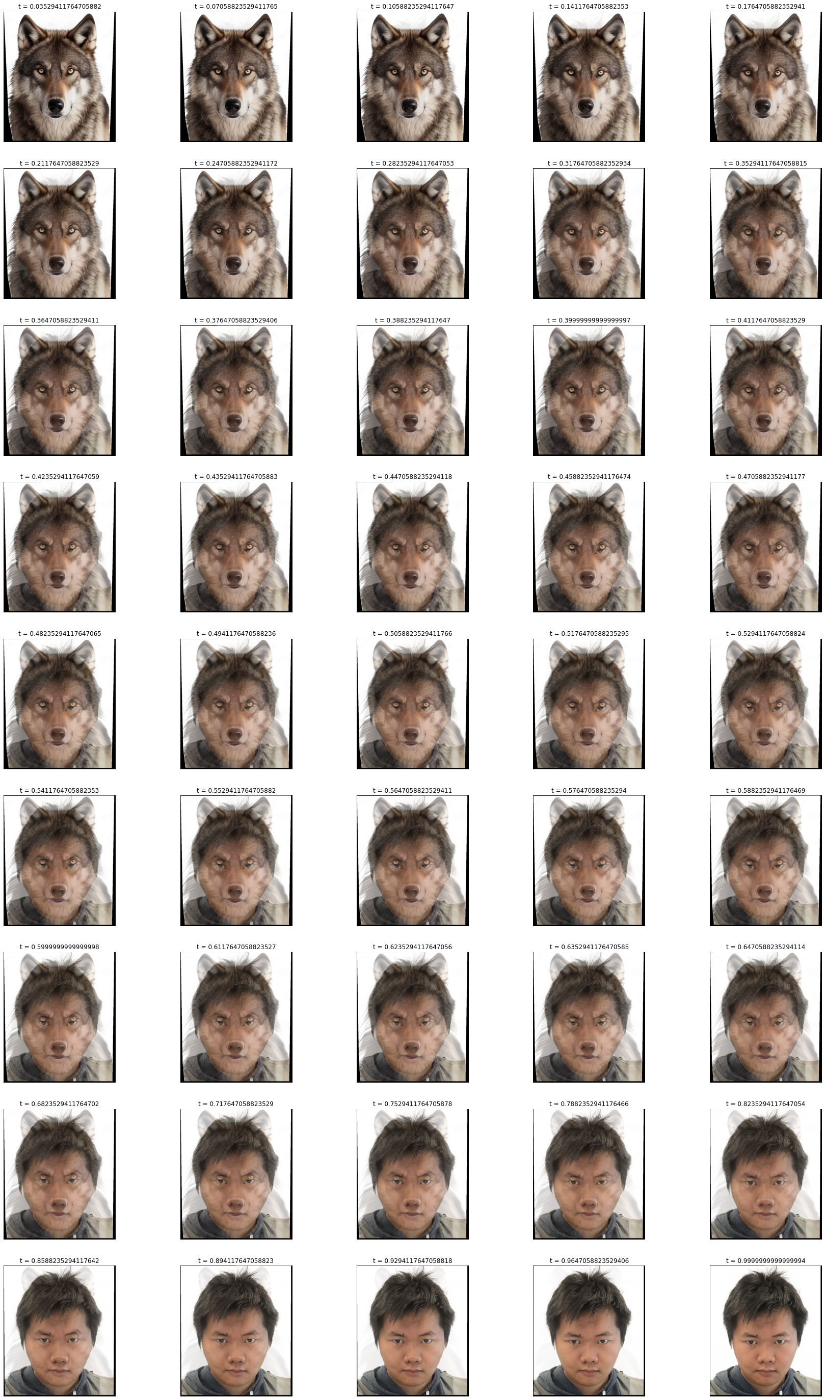
Prompt: At far, it looks like “a lithogram of a skull,” but upon close inspection, it’s actually “a lithogram of waterfalls”.

Prompt: At far, it looks like “tornado in a desert,” but upon close inspection, it’s actually “the face of a programmer”.
Check particualrly generated image 2.

Prompt: At far, it looks like “sunset in a desert,” but upon close inspection, it’s actually “a bar with dim lighting”.
Check particualrly generated image 3.

Project 5B: We Need to Go Deeper
The random seed used at here is always 0.
Implementing the UNet [1.1]
The UNet is an amalgation of several smaller convolution-based blocks. I implemented it. If you believe me, no need for further action. Else, here are some results.
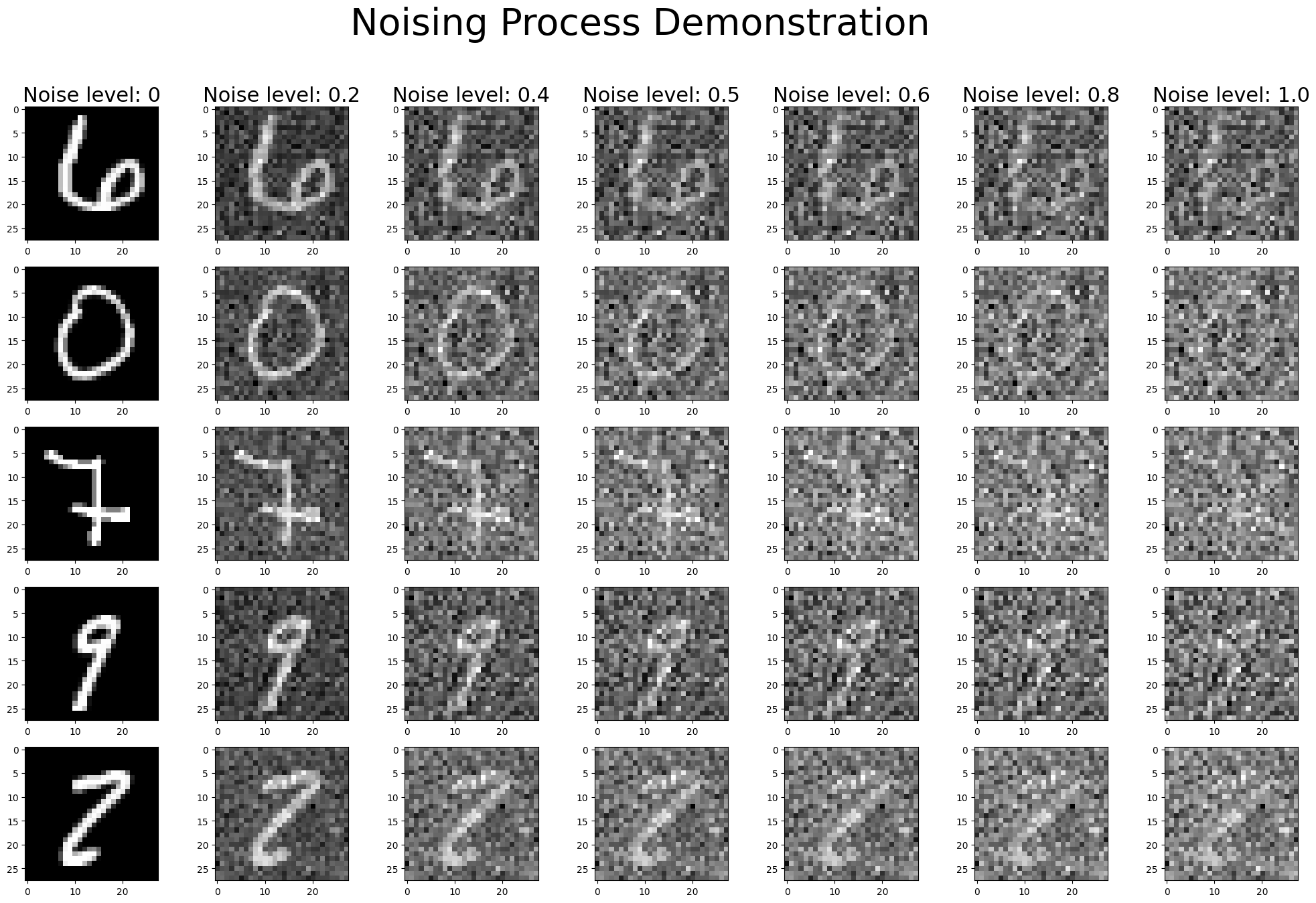
A demonstration for the noising process across choices of $\sigma$:
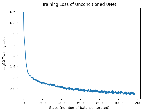
The training loss (logarithmically transformed) of the model:
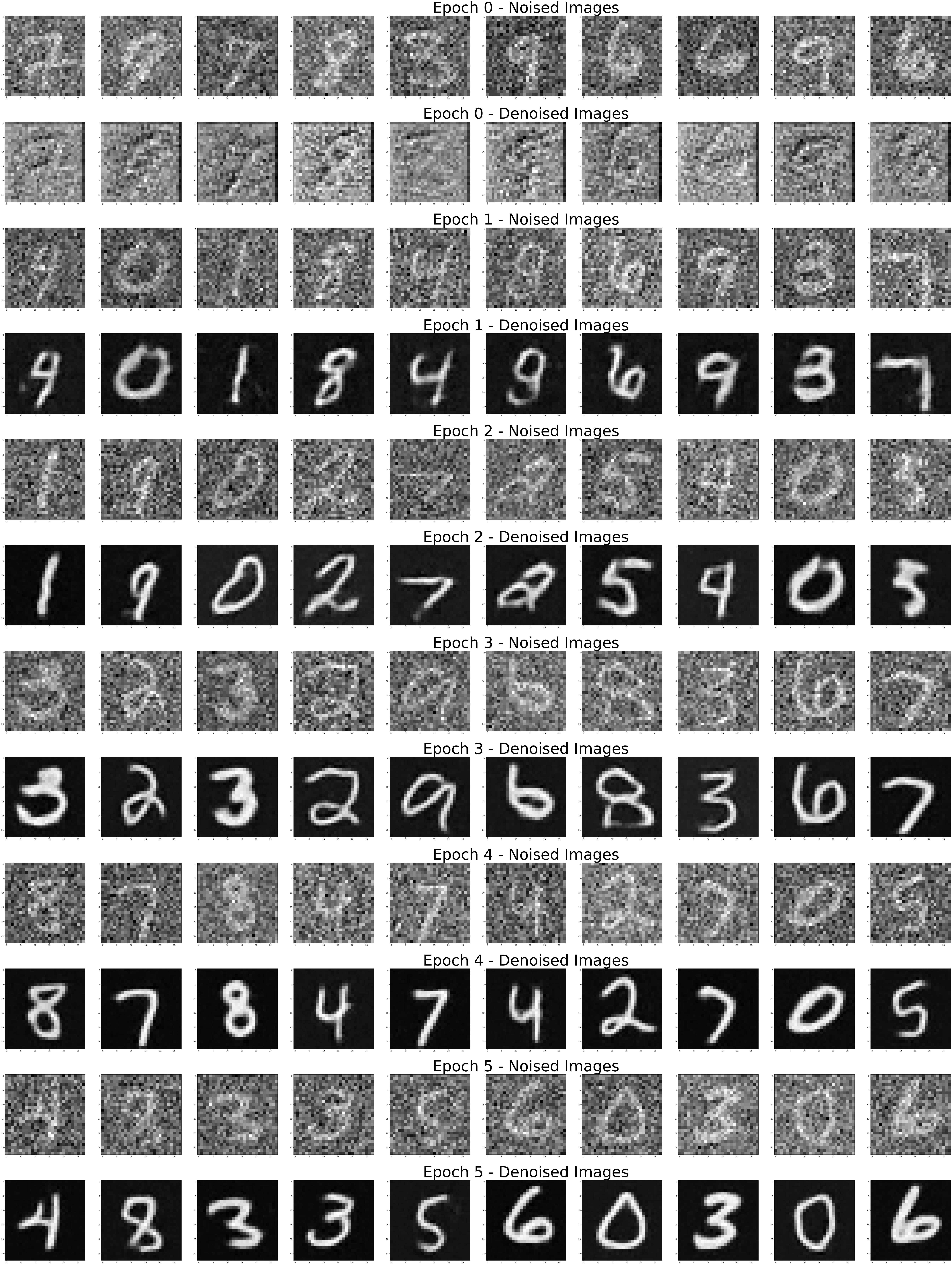
Some denoised results of the model:
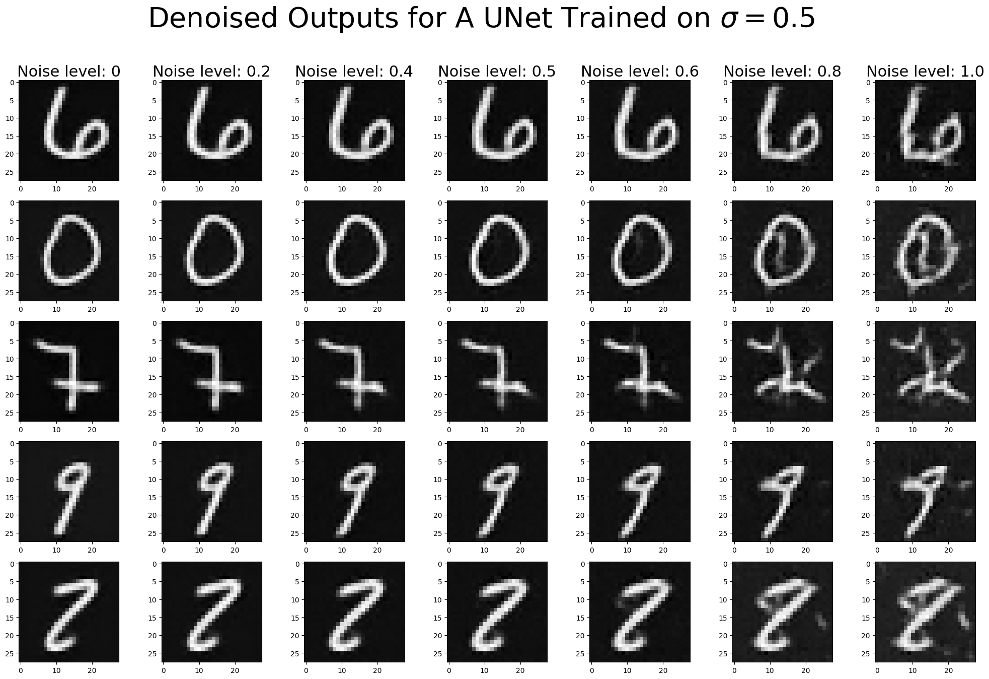
The performance of our denoise trained on $\sigma=0.5$ when it encounters a higher noise level:
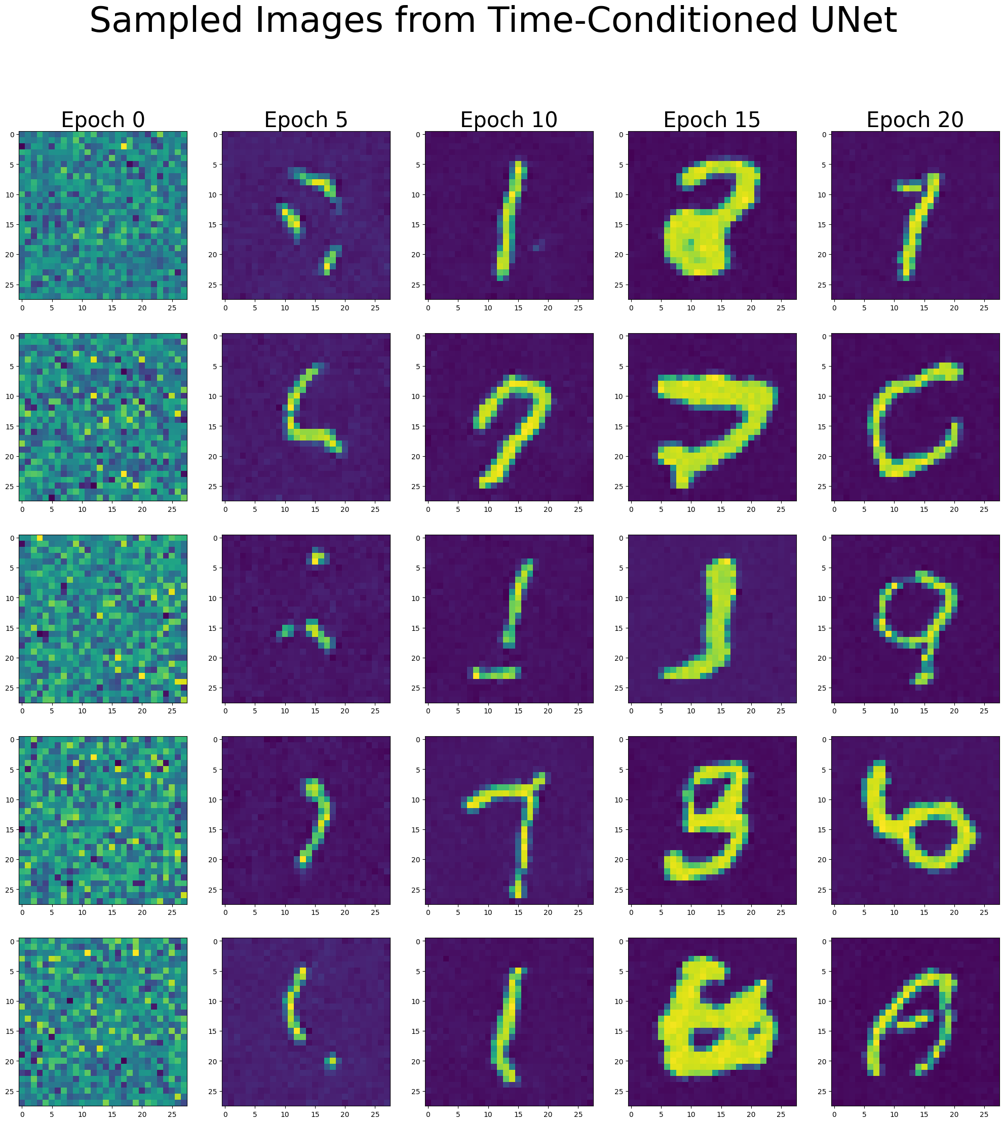
Time-Conditioned UNet [2.1, 2.2, 2.3]
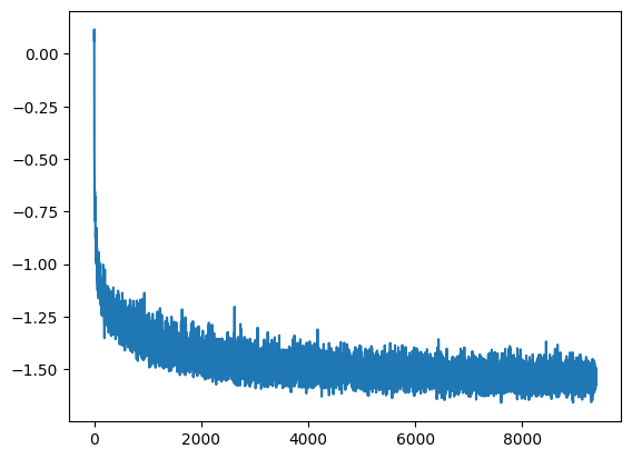
We can condition the UNet on timestep information to inform it how to denoise images provided the temporal situation of the denoising sequence. Particularly, this occurs with a fully connected block that takes timestep as an input.
The training loss of such model, logarithmically transformed, follows:
Its outputs:
Class-Conditioned UNet [2.4, 2.5]
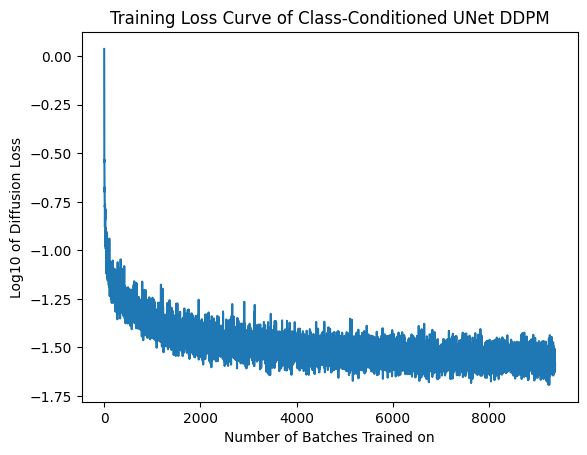
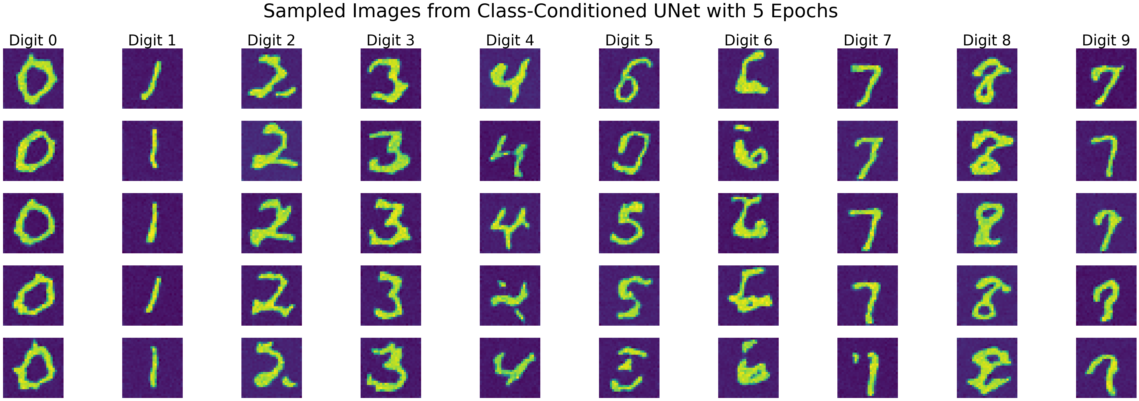
Similar to the theories of CFG, you can use class-conditioned embeddings to help diffusion models gear towards generating images of particular classes.
The training loss of such model, logarithmically transformed, follows:
Its outputs at the 5th epoch:
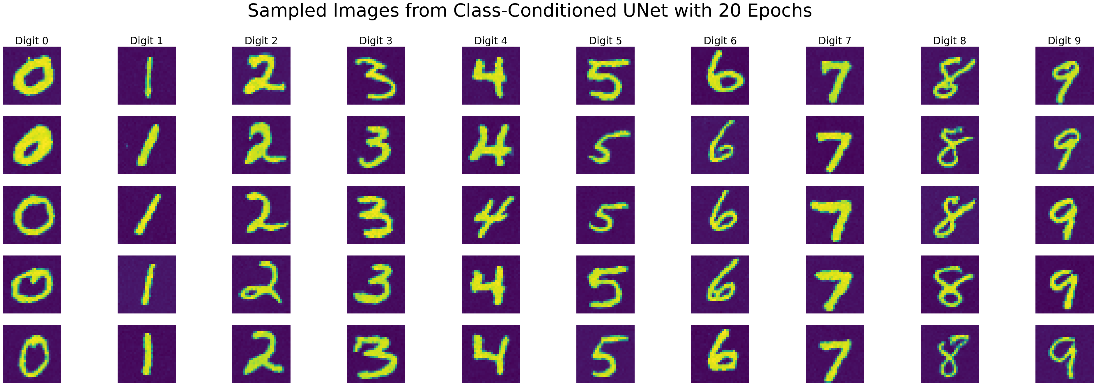
Its outputs at the 20th epoch:
